

2023/24 winter term
Being creative in physics
- Lecturer: Florian Marquardt
- 2,5 ECTS credit points
- 2 SWS
- Tuesday 18:00 - 19:30
2023 summer term
Machine Learning for Physicists
- Lecturer: Florian Marquardt
- One 90min seminar per week
- Thursday, 17:00 - 19:00
- Course website: https://pad.gwdg.de/s/Machine_Learning_For_Physicists_2023
Machine Learning for Physicists (Tutorial)
- Lecturer: Florian Marquardt
- One 90min tutorial per week
- Mondays, 16:00 - 18:00
2022/23 Winter term
Nanophysics and Quantum Optics
- Lecturer: Florian Marquardt
- One 90min seminar per week
- Tuesday, 13:30 - 15:00 (hybrid), starting 18th October 2022, end date 7th February 2023
Machine Learning for Quantum Technologies Discussion Group
- Lecturer: Florian Marquardt
- One 90min study group meeting per week
- Friday, 13:30 - 15:00 (hybrid), starting 21st October 2022, end date 10th February 2023
2022 Machine Learning for Physics - Hands-on Programming Group
- Lecturer: Florian Marquardt, Matteo Puviani
- One 90min lecture per week
- Friday, 13:30 - 15:00 (online), starting 29th April 2022, end date 29th July 2022
Nanophysics and Quantum Optics Seminar
- Lecturer: Florian Marquardt, Matteo Puviani
- One 90min lecture per week
- Tuesday, 13:30 - 15:00 (online), starting 26th April 2022, end date 26th July 2022
2021/22 Advanced Machine Learning for Physics and Scientific Discovery
- Lecturer: Florian Marquardt
- 10 ECTS credit points
- 4 SWS
- Monday 18:00 - 19:30 (online), starting 18th October 2021, end date 9th February 2022
For more information, e. g. on registration for the course and a course summary, please visit the lecture website.
2021 Machine Learning for Physicists
- Lecturer: Florian Marquardt
- 5 ECTS credit points
- One 90min lecture per week
- Monday 18:00 - 19:30 (online), starting 12 April 2021, end date 12 July 2021
For more information, e. g. on registration for the course and a course summary, please visit the lecture website.
2020/21 Foundations of Quantum Mechanics

- Lecturer: Florian Marquardt
- 5 ECTS credit points
- One 90min lecture per week
- Monday 18:00 - 19:30 (online), starting 2 November 2020
- For more information, e. g. on registration for the course and a course summary, please visit the lecture website.
2020 Machine Learning for Physicists
Introduction to deep neural networks and other machine learning techniques, for physicsts.
Online course ('inverted classroom'), running from April 21 to August 4, every Tuesday at 6pm.
Please see the official course website: "Machine Learning for Physicists 2020"
2019 Machine Learning for Physicists
Please visit the official domain machine-learning-for-physicists.org, where we collected all the videos and slides from the 2017 Machine Learning for Physics Lecture Series for quick download!
Basic Information about this lecture series
- Contact: florian.marquardt@mpl.mpg.de
- 2 hours/week, 5 ECTS credit points
- UnivIS
- Exam: 9th August 2019, 10:00 - 12:00, Lecture Hall G, Staudtstraße 5, 91058 Erlangen
- Repeat exam: 4th October 2019, 10:00 - 12:00 Lecture Hall F, Staudtstraße 5, 91058 Erlangen
Description: This is a course introducing modern techniques of machine learning, especially deep neural networks, to an audience of physicists. Neural networks can be trained to perform many challenging tasks, including image recognition and natural language processing, just by showing them many examples. While neural networks have been introduced already in the 50s, they really have taken off in the past decade, with spectacular successes in many areas. Often, their performance now surpasses humans, as proven by the recent achievements in handwriting recognition and in winning the game of 'Go' against expert human players. They are now also being considered more and more for applications in physics, ranging from predictions of material properties to analyzing phase transitions.
Contents: We will cover the basics of neural networks (backpropagation), convolutional networks, autoencoders, restricted Boltzmann machines, and recurrent neural networks, as well as the recently emerging applications in physics. Time permitting, we will address other topics, like the relation to spin glass models, curriculum learning, reinforcement learning, adversarial learning, active learning, "robot scientists", deducing nonlinear dynamics, and dynamical neural computers.
Prerequisites: As a prerequisite you will only need matrix multiplication and the chain rule, i.e. the course will be understandable to bachelor students, master students and graduate students. However, knowledge of any computer programming language will make it much more fun. We will sometimes present examples using the 'python' programming language, which is a modern interpreted language with powerful linear algebra and plotting functions.
Book: The first parts of the course will rely heavily on the excellent and free online book by Nielsen: "Neural Networks and Deep Learning"
Software: Modern standard computers are powerful enough to run neural networks in a reasonable time. The following list of software packages helps to keep the programming effort low (it is possible to implement advanced structures like a deep convolutional neural network in only a dozen lines of code, which is quite amazing):
- Python is a widely used high-level programming language for general-purpose programming; both Theano and Keras are Python moduls. We highly recommend the usage of the 3.x branch (cmp. Python2 vs Python3).
- TensorFlow is a package for dataflow and differentiable programming, developed by Google. It is a symbolic math library for a broad range of tasks, including machine learning applications such as neural networks. For that purpose, TensorFlow provides the low-level tools (multi-dimensional arrays, convolutional layers, efficient computation of the gradient, ...).
- Keras is a high-level framework for neural networks, running on top of TensorFlow. Designed to enable fast experimentation with deep neural networks, it focuses on being minimal, modular and extensible.
- Matplotlib is a plotting library for the Python programming language. We use it to visualize our results.
- Jupyter is a browser-based application that allows to create and share documents that contain live (Python) code, equations, visualizations and explanatory text. So, Jupyter serves a similar purpose like Mathematica notebooks.
All the software above is open source and freely available for a large number of platforms. See also the installation instructions.
Links
- Eight inspirational applications of deep learning, from automatic colorization of images to playing games, by Jason Brownlee
- Deep Learning Examples, a great set of slides on a large array of recent deep learning applications, by Lukas Masuch
- A Hacker's Guide to Neural Networks: a slightly unconventional, practical introduction to backpropagation, by Andrej Karpathy
- The Unreasonable Effectiveness of Recurrent Neural Networks, on creating fake Shakespeare plays or Wikipedia articles by training neural networks on them (character by character); by Andrej Karpathy
2017/18 Machine Learning for Physicists
This seminar is a follow-up to the lecture of the summer term of 2017.
Students will be asked to present modern research articles on machine learning, especially those that address the application of machine learning techniques to questions in physics (and in the natural sciences in general).
- Tentative schedule: Mondays, 18:00-20:00 (I'm choosing this slot so that a maximum number of students may participate if they like to)
- First meeting: Monday, October 23.
- Where: Lecture hall F
- Also look for the studon-group
- Lecturer/Advisor: Florian.Marquardt@fau.de
Schedule:
- 30.10.: Florian Unger, Neural Turing Machine
- 13.11.: Matthias Zürl, Go
- 20.11.: Alexander Blania, Inverse Imaging or Bell Inequalities
- 27.11.: Manyu Wen, Neural Hybrid Computing
- 6.12. (Wednesday!): Tim Stüven, Predicting Dynamics of 2D objects or Bell inequalities & Ankan Bag, Coherent Nanophotonic Circuits
- 18.12.: Bystrik Matas, Renormalization Group and Neural Networks or Quantum Many-Body Dynamics
- 15.1.: Philip Thalhammer, Detection of Gravitational Lensing
- 22.1.: David Böhringer, Toxic Materials or Face of Crystals & Felix Lammermann, Superconducting Transition Temperatures
- 29.1.: Jasmin Graf, Active Learning for Quantum Experiments
- 7.2. (Wednesday!): Timo Niehoff, Phase Transitions by Confusion and Sourav Chatterjee
2017: Quantum Mechanics (Theory) - Integrated course 1 (IK-1)
- Lecturer: Andrea Aiello
- Contact: Andrea Aiello
- Lectures: Monday 13:30 - 15:30, SR 01.683; Tuesday, Thursday, 10:00 - 12:00, SR 01.683; Wednesday 11:00 - 13:00, SR 01.683
- Exercises: Thursday 13:00 - 16:00, SR 00.103
Preliminary program
Lecture notes
- Lectures 1-2 (PDF)
- Lecture 3 (PDF)
- Lectures 4-5 (PDF)
- Lectures 5-6 (PDF)
- Lecture 7 (PDF)
- Addendum to Lecture 7 (PDF)
- Lecture 8 (PDF)
- Lecture 9 (PDF)
- Lecture 10 (PDF)
- Lecture 11 (PDF)
- Lecture 12 (PDF)
- Lecture 13 (PDF)
- Lecture 14 (PDF)
- Addendum to Lecture 14 (PDF)
- Compendium on Angular Momentum (PDF)
- Lecture 15 (PDF)
- Lecture 16 (PDF)
- Lecture 17 (PDF)
- Lecture 18 (PDF)
- Lecture 19 (PDF)
- Lecture 20 (PDF)
- Lecture 21 (PDF)
- Examples for Lecture 21 (PDF)
- Addendum to Lecture 21 (PDF)
- Lecture 22 (PDF)
- Lecture 23 (PDF)
- Singular Value Decomposition (PDF)
Exercise sheets
- Worksheet 1 (PDF)
- Worksheet 2 (PDF)
- Addendum to Worksheet 2 (PDF)
- Worksheet 3a (PDF)
- Worksheet 3b (PDF)
- Worksheet 4 (PDF)
- Worksheet 5 (PDF)
- Worksheet 6 (PDF)
Quotations
- From p. 414 of: Peter D. Lax, Functional analysis, (John Wiley & Sons, Inc., 2002)
The theory of self-adjoint operator was created by von Neumann to fashion a framework for quantum mechanics. [...] I recall in the summer of 1951 the excitement and elation of von Neumann when he learned that Kato has proved the self-adjointness of the Schroedinger operator associated with the helium atom. And what do the physicists think of these matters? In the 1960s Friedrichs met Heisenberg, and used the occasion to express to him the deep gratitude of the community of mathematicians for having created quantum mechanics, which gave birth to the beautiful theory of operators in Hilbert space. Heisenberg allowed that this was so; Friedrichs then added that the mathematicians have, in some measure, returned the favor. Heisenberg looked noncommittal, so Friedrichs pointed out that it was a mathematician, von Neumann, who clarified the difference between a self-adjoint operator and one that is merely symmetric."What's the difference", said Heisenberg.
- From p. vii of: Josef M. Jauch, Foundations of Quantum Mechanics, (Addison-Wesley Publishing Company, Inc., 1968)
Contrary to a widespread belief, mathematical rigor, appropriately applied, does not necessarily introduce complications. In physics it means that we replace a traditional and often antiquated language by a precise but necessarily abstract mathematical language, with the result that many physically important notions formerly shrouded in a fog of words become crystal clear and of surprising simplicity.
- From p. vii-viii of: Cornelius Lanczos, The variational principles of mechanics, 4th ed. (Dover Publications, Inc., 1970)
Many of the scientific treatises of today are formulated in a half-mystical language, as though to impress the reader with the uncomfortable feeling that he is in the permanent presence of a superman.
Bibliography
- R. Shankar, Principles of Quantum Mechanics, 2nd ed. (Springer, 1994) - basic
- R. L. Liboff, Introductory Quantum Mechanics, (Addison-Wesley, 1980) - basic
- S. Gasiorowicz, Quantum Physics, 3rd ed. (John Wiley & Sons, 2003) - basic
- D. J. Griffiths, Introduction to Quantum Mechanics, 2nd ed. (Cambridge University Press, 2016) - basic
- E. Merzbacher, Quantum Mechanics, 3rd ed. (John Wiley & Sons, 1998) - intermediate
- J. J. Sakurai, Modern Quantum Mechanics, 3rd ed. (The Benjamin/Cummings Publishing Company, Inc., 1985) - intermediate
- W. Greiner, Quantum Mechanics, An Introduction, 4th ed. (Springer-Verlag, 2001)- intermediate
- C. Cohen-Tannoudji, B. Diu, F. Lalöe, Quantum Mechanics, Vol. I and Vol. II (John Wiley & Sons, 2005) - intermediate/advanced
- G. Baym, Lectures on Quantum Mechanics, (Westview Press, 1990) - intermediate/advanced
- L. D. Landau, L. M. Lifshitz, Quantum Mechanics: Non-Relativistic Theory (Volume 3), 3rd ed. (Butterworth-Heinemann, 1981) - intermediate/advanced
- A. Messiah, Quantum Mechanics, (Dover Publications, Inc., 1999) - intermediate/advanced
- S. Weinberg, Lectures on Quantum Mechanics, 1st ed. (Cambridge University Press, 2013) - intermediate/advanced
- J. Schwinger, Quantum Mechanics, (Springer, 2001) - advanced
- A. Galindo, P. Pascual, Quantum Mechanics I and II, (Springer, 1990) - advanced
- A. Peres, Quantum Theory: Concepts and methods, (Kluver Academic Publishers, 1995) - advanced
- A. Sudbery, Quantum mechanics and the particles of nature, 3rd ed. (Cambridge University Press, 1986) - alternative
- T. F. Jordan, Quantum mechanics in simple matrix form, (Dover Publications, Inc., 1986) - alternative
- T. F. Jordan, Linear Operators for Quantum Mechanics, (Dover Publications, Inc., 1997) - mathematics/mathematical physics
- C. Lanczos, Linear Differential Operators, (Martino Publishing, 2012) - mathematics/mathematical physics
- I. S. Gradshteyn, I. M. Ryzhik, Table of Integrals, Series, and Products, 5th ed. (Academic Press, 1994) - mathematics/mathematical physics
- A. Papoulis, S. U. Pillai, Probability, Random Variables and Stochastic Processes, 4th ed. (McGraw-Hill, 2002) - probability theory
- J. M. Jauch, Are Quanta Real? (Indiana University Press, 1989) - didactic/history
- G. Gamow, Thirty years that shook physics. The story of quantum theory, (Dover Publications, Inc., 1985) - didactic/history
Online resources
- The Feynman Lectures on Physics Online edition of "The Feynman Lectures on Physics"
- NIST Digital Library of Mathematical Functions Online library of mathematical functions
- Wolfram Online Integral Calculator Online integral calculator
- WolframAlpha Online mathematics, physics and more
- Quantum Physics I Allan Adams, Matthew Evans, and Barton Zwiebach. 8.04 Quantum Physics I. Spring 2013. Massachusetts Institute of Technology: MIT OpenCourseWare, https://ocw.mit.edu. License: Creative Commons BY-NC-SA.
- Quantum Physics II Barton Zwiebach. 8.05 Quantum Physics II. Fall 2013. Massachusetts Institute of Technology: MIT OpenCourseWare, https://ocw.mit.edu. License: Creative Commons BY-NC-SA.
- Quantum Physics III Aram Harrow. 8.06 Quantum Physics III. Spring 2016. Massachusetts Institute of Technology: MIT OpenCourseWare, https://ocw.mit.edu. License: Creative Commons BY-NC-SA.
- C. Patrignani et al. (Particle Data Group), Chin. Phys. C 40, 100001 (2016). See table 44 "Clebsch-Gordan Coefficients, Spherical Harmonics, and d Functions" in the section "Mathematical Tools"
- Probability, Mathematical Statistics, Stochastic Processes A great website devoted to probability, mathematical statistics, and stochastic processes.
Relevant didactic articles
- Nine formulations of quantum mechanics, American Journal of Physics 70, 288 (2002) Quantum mechanics can be formulated in many different and equivalent ways. In this article the authors present a brief review (with annotated bibliography) of nine different formulations of quantum mechanics.
- On quantum theory, Eur. Phys. J. D (2013) 67: 238 One of the most lucid and scientifically honest recent expositions of quantum theory by B-G. Englert, one of the last PhD students of Julian Schwinger. Some of the so-called paradoxes of quantum mechanics are analyzed and deconstructed.
- What is a state in quantum mechanics? American Journal of Physics 72, 348 (2004) A very interesting read about the actual meaning of a quantum state. Especially relevant is the second part of section II about possible instantaneous action-at-a-distance effects. Unfortunately the article suffer from numerous typos, please read also the "Erratum".
- What is a state vector? American Journal of Physics 52, 644 (1984) This and the next article are from the late Asher Peres, one of the most profound modern thinkers about quantum mechanics (see his celebrated book above). In this article Peres shows that "[...] a state vector represents a procedure for preparing or testing one or more physical systems. No "quantum paradoxes" ever appear in this interpretation."
- When is a quantum measurement? American Journal of Physics 54, 688 (1986) In this article Peres gives a clear analysis of a measurement in quantum mechanics and discuss the so-called "collapse" of the wavefunction.
- Is There a Quantum Measurement Problem? Phys. Rev. D 5, 1028 (1972) Another transparent analysis of the measurement problem in quantum mechanics. Note that the presentation of the subject given in this article is a bit advanced.
- Self‐adjointness and spontaneously broken symmetry, American Journal of Physics 45, 823 (1977) This article and the next two deal with the concept of self-adjoint extensions of operators. In this paper the author present a very clear and interesting physical model showing that, contrary to popular belief, the distinction between Hermitian, self-adjoint and essentially self-adjoint operators has physical roots.
- Self-adjoint extensions of operators and the teaching of quantum mechanics, American Journal of Physics 69, 322 (2001) A clear and concise exposition of the notion of self-adjoint extensions of operators, deficiency indexes and von Neumann theorem, at undergraduate level.
- Operator domains and self-adjoint operators, American Journal of Physics 72, 203 (2004) In the intention of the authors, the purpose of this paper is to supplement and expand the presentation given in the previous article. Many interesting examples are given.
Material for exercises
- Quantum Physics I - exercises Quantum Physics I, Allan Adams, Matthew Evans, and Barton Zwiebach. 8.04 Quantum Physics I. Spring 2013. Massachusetts Institute of Technology: MIT OpenCourseWare, https://ocw.mit.edu. License: Creative Commons BY-NC-SA.
2017 Machine Learning for Physicists
Basic Information about this Lecture Series
- Contact: Florian.Marquardt@fau.de
- 2 hours/week, 5 ECTS credit points
- Mailing list: If you are a regular student, please join the studon course "Machine Learning for Physicists 2017". If you are a PhD student (without a studon account), please send an email to marquardt-office@mpl.mpg.de (Gesine Murphy), with the subject line "MACHINE LEARNING". Then you will be added to a mailing list.
- Time/place: Monday 18:00-20:00 and Thursday, 18:00-20:00. (though not every week; see schedule below!)
- Video: Videos of the lectures (made available weekly)
- First lecture: Monday, May 8, 2017; 18:00, lecture hall F
- Second lecture: Thursday, May 11, 18:00, lecture hall D (!)
- Third lecture: Monday, May 22, 18:00, lecture hall G
- Further lecture times: See time table below. From now on, we will always be in lecture hall G.
- EXAM: Written exam August 9th, 10:00-12:00. Lecture hall D. Please be there a few minutes earlier! During the exam, one A4 page of notes (handwritten by yourself, both sides if needed) is allowed, but nothing more.
- REPEAT EXAM: Written exam, Wednesday, October 11, 10:00-12:00. Lecture hall B. Please be there a few minutes earlier! During the exam, one A4 page of notes (handwritten by yourself, both sides if needed) is allowed, but nothing more.
- Example Questions: Here is a test problem set, for practice.
- Repetition exam on October 11, 10:00-12:00, lecture hall E.
Description: This is a course introducing modern techniques of machine learning, especially deep neural networks, to an audience of physicists. Neural networks can be trained to perform many challenging tasks, including image recognition and natural language processing, just by showing them many examples. While neural networks have been introduced already in the 50s, they really have taken off in the past decade, with spectacular successes in many areas. Often, their performance now surpasses humans, as proven by the recent achievements in handwriting recognition and in winning the game of 'Go' against expert human players. They are now also being considered more and more for applications in physics, ranging from predictions of material properties to analyzing phase transitions.
Contents: We will cover the basics of neural networks (backpropagation), convolutional networks, autoencoders, restricted Boltzmann machines, and recurrent neural networks, as well as the recently emerging applications in physics. Time permitting, we will address other topics, like the relation to spin glass models, curriculum learning, reinforcement learning, adversarial learning, active learning, "robot scientists", deducing nonlinear dynamics, and dynamical neural computers.
Prerequisites: As a prerequisite you will only need matrix multiplication and the chain rule, i.e. the course will be understandable to bachelor students, master students and graduate students. However, knowledge of any computer programming language will make it much more fun. We will sometimes present examples using the 'python' programming language, which is a modern interpreted language with powerful linear algebra and plotting functions.
Book: The first parts of the course will rely heavily on the excellent and free online book by Nielsen: "Neural Networks and Deep Learning"
Software: Modern standard computers are powerful enough to run neural networks in a reasonable time. The following list of software packages helps to keep the programming effort low (it is possible to implement advanced structures like a deep convolutional neural network in only a dozen lines of code, which is quite amazing):
- Python is a widely used high-level programming language for general-purpose programming; both Theano and Keras are Python moduls. We highly recommend the usage of the 3.x branch (cmp. Python2 vs Python3).
- Theano is a numerical computation library for Python. In Theano, computations are expressed using a NumPy-like syntax and compiled to run efficiently on either CPU or GPU architectures. Therefore, Theano provides the low-level tools (multi-dimensional arrays, convolutional layers, efficient computation of the gradient, ...) needed to implement artificial neural networks.
- Keras is a high-level framework for neural networks, running on top of Theano. Designed to enable fast experimentation with deep neural networks, it focuses on being minimal, modular and extensible.
- Matplotlib is a plotting library for the Python programming language. We use it to visualize our results.
- Jupyter is a browser-based application that allows to create and share documents that contain live (Python) code, equations, visualizations and explanatory text. So, Jupyter serves a similar purpose like Mathematica notebooks.
All the software above is open source and freely available for a large number of platforms. See also the Installation instructions section below.
Lecture Notes and Files
- PDF Slides Lecture 1 (8.5.2017)
- PDF Slides Lecture 2 v2 (11.5.2017)
- PDF The Python Cheat Sheet (many useful examples, on 2 pages)
- python code for visualizing the output of a multilayer network (demonstrates batch processing and produces a nice picture)
- PDF Slides Lecture 3 v4 (22.5.2017)
- python code for full backpropagation algorithm (without example)
- Jupyter Notebook for backpropagation and example (as in the lecture; Note: After downloading, in some browsers, you may have to remove the ending ".txt", such that the file has the ending ".ipynb"; then use "jupyter notebook" and open the file!)
- PDF Slides Lecture 4 v1 (29.5.2017)
- Jupyter Notebook for Image Representation, also download the sample pictures: Smiley and Emmy (if you want to use your own image, use a square image or revise the code!)
- Jupyter Notebook Image Representation with Keras (uses keras, otherwise the same functionality as above)
- PDF Slides Lecture 5 v1 (8.6.2017)
- Jupyter Notebook Handwritten Digit Recognition with Keras (needs MNIST data file, see below)
- MNIST training images (17 MB, in a compressed format which can be read by the notebook above); Note: This is the version available from Nielsen's website for his deep learning book: it is contained in the code package for that book. The original version is available from Yann LeCun's website, together with a list of training results for various machine learning approaches!
- PDF Slides Lecture 6 v1 (19.6.2017)
- Autoencoder Example (jupyter notebook)
- MNIST recognition with a convolutional net
- PDF Slides Lecture 7 v1 (26.6.2017) (10 MB due to some large example images!)
- PDF Slides Lecture 8 v1 (29.6.2017)
- Jupyter Notebook: Simple LSTM examples (a network that memorizes a number and recalls it later upon request, and a network that counts down)
- PDF Slides Lecture 9 v1 (3.7.2017)
- Convolutional Image Recognition - jupyter notebook for tutorial on 6.7. (simple image classification)
- PDF Slides Lecture 10 v1 (10.7.2017)
- Simple Reinforcement Learning Example - "Walker/Target" example, as explained in the lectures (jupyter notebook).
- PDF Slides Lecture 11 v1 (17.7.2017)
- PDF Slides Lecture 12 v1 (24.7.2017)
Installation instructions
The following instructions should be quite detailed and easy to follow. If you nevertheless encounter a problem which you cannot solve for yourself, please write an email to Thomas Foesel.
Note: the monospaced text in this section are commands which have to be executed in a terminal.
- for Linux/Mac: The terminal is simply the system shell. The "#" at the start of the line indicates that root privileges are required (so log in as root via su, or use sudo if this is configured suitably), whereas the commands starting with "$" can be executed as a normal user.
- for Windows: Type the commands into the Conda terminal which is part of the Miniconda installation (see below).
Installing Python, Theano, Keras, Matplotlib and Jupyter
In the following, we show how to install these packages on the three common operating systems. There might be alternative ways to do so; if you prefer another one that works for you, this is also fine, of course.
- Linux
- Debian/Mint/Ubuntu/...
- # apt-get install python3 python3-dev python3-matplotlib python3-nose python3-numpy python3-pip
- # pip3 install jupyter keras Theano
- openSUSE
- # zypper in python3 python3-devel python3-jupyter_notebook python3-matplotlib python3-nose python3-numpy-devel
- # pip3 install Theano keras
- Debian/Mint/Ubuntu/...
- Mac
- Download the installation script for the Miniconda collection (make sure to select Python 3.x, the upper row). In the terminal, go into the directory of this file ($ cd ...) and run # bash Miniconda3-latest-MacOSX-x86_64.sh.
- Because there are more recent Conda versions than on the website, update it via conda update conda.
- Create a Conda environment with
$ conda create --name neuralnets python=3.5
(note that keras does not run on python 3.6 yet) and activate it via
$ source activate neuralnets. - $ conda install numpy scipy mkl nose sphinx theano pygpu yaml hdf5 h5py jupyter matplotlib
- $ pip install keras
- Windows
- Download and install the Miniconda collection (make sure to select Python 3.x, the upper row).
- Because there are more recent Conda versions than on the website, update it via conda update conda.
- Create a Conda environment with
conda create --name neuralnets python=3.5
(note that keras does not run on python 3.6 yet) and activate it via
activate neuralnets. - conda install jupyter h5py hdf5 libpython m2w64-toolchain matplotlib mkl-service nose nose-parameterized numpy scipy sphinx theano yaml
- pip install keras
Configuration: protecting Jupyter
Important: If you intend to run Jupyter on a multi-user system (like the CIP pool), it is absolutely necessary to protect it against arbitrary code execution by other users. The instructions can be found here.
Configuration: tell Keras to use the Theano backend
- Load Keras into Python (this command will probably fail as it tries to load TensorFlow, but this is OK. Its purpose is to initialize the ".keras" folder):
- on Linux: $ python3 -c "import keras"
- on Mac: $ source activate neuralnets; python -c "import keras"
- on Windows:
activate neuralnets
python -c "import keras"
- edit file ".keras/keras.json" in your home directory: replace "tensorflow" with "theano". To do that,
- on Linux/Mac: open file "~/.keras/keras.json" in your home directory with your preferred text editor (either with command line editors like $ vi ~/.keras/keras.json, $ emacs ~/.keras/keras.json and $ nano ~/.keras/keras.json, or any graphical text editor)
- on Windows:
cd %USERPROFILE%
notepad .keras/keras.json
Minimal examples
After the previous steps, the following scripts should work for you :
Minimal example for Matplotlib
To check this, download the scripts, rename the file extension from ".txt" to ".py", and execute them
- on Linux: $ python3 <script.py>, e.g. $ python3 theano_minimal.py
- on Mac (with Miniconda):
- $ source activate neuralnets (has to be done once in each new shell session)
- $ python <script.py>, e.g. $ python theano_minimal.py
- on Windows (with Miniconda):
- activate neuralnets (has to be done once in each new shell session)
- python.exe <script.py>, e.g. $ python.exe theano_minimal.py (in the Conda shell, also python <script.py> should work)
In the same way, you should also be able to execute your own Python scripts. If you call $ python3/$ python/python.exe without an argument, an interactive session is started, i.e. you can directly enter Python commands into the terminal.
In addition, you should be able to start a Jupyter notebook via $ jupyter notebook (will automatically open a browser tab where you can work).
Links
- Eight inspirational applications of deep learning, from automatic colorization of images to playing games, by Jason Brownlee
- Deep Learning Examples, a great set of slides on a large array of recent deep learning applications, by Lukas Masuch
- A Hacker's Guide to Neural Networks: a slightly unconventional, practical introduction to backpropagation, by Andrej Karpathy
- The Unreasonable Effectiveness of Recurrent Neural Networks, on creating fake Shakespeare plays or Wikipedia articles by training neural networks on them (character by character); by Andrej Karpathy
2016: Foundations of Quantum Mechanics
- Lecturer: Florian Marquardt
- Contact: Florian Marquardt
- 10 ECTS credit points
- Two 90min lectures per week, plus one 90min tutorial class
- Monday 18:00-19:30 lecture hall F
- Friday 16:00-17:30 lecture hall F
- Tutorial: Wednesday 16:15-17:45 SR 01.779 (sometimes shifted to 18:00-19:30)
Overview
Have you ever wondered about the mysterious "collapse of the wave function" or the "wave-particle duality"? Does Schrödinger's cat make you uneasy? Do you have a feeling that there could be a deeper, more 'microscopic' theory underlying Quantum Mechanics? Do you believe that trajectories are ruled out by Quantum Mechanics? Are you confused by the concept of spin or by fermions vs. bosons? Do you want to learn how the founding fathers' "Gedankenexperiments" are now routinely realized in the labs?
This lecture series addresses questions related to the foundations of Quantum Mechanics. Topics will include:
- Bell's inequalities and Entanglement
- Measurements
- Decoherence and the quantum-to-classical crossover
- Interpretations of Quantum Mechanics (including Bohm's pilot wave and Nelson's Stochastic Quantization)
- Extensions of Quantum Mechanics (for example "spontaneous localization")
- Geometric phases (Aharonov-Bohm effect and all that)
- Particle statistics
- Quantum electrodynamics (including vacuum effects, renormalization, and Stochastic Electrodynamics)
- Relativistic quantum mechanics
The lectures require knowledge as obtained in a standard first course on Quantum Mechanics (more background will be beneficial but not absolutely needed). Master-level students and PhD students (as well as postdocs) will probably get the most out of this course.
Videos
The lectures have been recorded on video in 2013 and put online during the term as they become available. You can find them on the Erlangen server:
Lecture Notes
From the 2013 version, may be slightly modified in 2016.
- Lecture Notes Part 1 (PDF) (Introduction, Bell's inequalities and entanglement; Pages 1-46)
- Lecture Notes Part 2 (PDF) (Bell tests, entanglement, measurement; Pages 47-78)
- Update: The trio of loophole-free Bell tests from 2015 – Delft experiment, Vienna experiment, and Boulder experiment
- Lecture Notes Part 3 (PDF) (Weak measurements, decoherence; Pages 79-119)
- Lecture Notes Part 4 (PDF) (Interpretations of Quantum Mechanics, Extensions of Quantum Mechanics; Pages 120-168)
- Lecture Notes Part 5 (PDF) (Geometrical Phases, Particle Statistics, QED, Dirac Equation; Pages 169-231)
Original Literature
Note: Most of these papers are in German. English translations may be found in the book 'B. L. van der Waerden, editor, Sources of Quantum Mechanics (Dover Publications, 1968) ISBN 0-486-61881-1.
- On the Theory of Quanta, PhD thesis of Louis-Victor de Broglie (1924), English translation by A. Kracklauer: Download e-book
- Heisenberg's original matrix mechanics - This is the work that created the modern theory of quantum mechanics (Heisenberg 1925). Heisenberg wanted to tackle the question of how to predict correctly the intensities of atomic transition lines, as Bohr had already clarified how to obtain the transition frequencies. Heisenberg began by noticing that, according to Bohr, the correct quantum transition frequencies do not depend just on the current state of motion (as do the frequencies of emitted radiation for a classical orbit), but rather on two states (initial and final). Likewise, in classical theory, the intensities of emitted radiation would be given by the squares of the Fourier amplitudes of the oscillating dipole moment for a given orbit. In an ingenious step, Heisenberg then postulated that instead of a set of Fourier amplitudes for a given orbit (enumerated by one index), one would have to introduce a set of amplitudes depending on two indices, one for the initial, the other for the final state. He assumed that the equations of motion for those amplitudes looked formally the same as in classical theory (Heisenberg equations of motion). The last crucial ingredient is the commutation relation. This he derived by looking at the linear response of an electron to an external perturbation (essentially deriving something like Kubo's formula, containing the commutator) and then demanding that the short-time response would be always that of a free, classical electron. This fixes the commutator between position and momentum. Thus was born matrix mechanics. He applied this immediately to the harmonic oscillator and also dealt with the anharmonic oscillator using perturbation theory. See also Heisenberg's Nobel Lecture from 1933 to learn more about his view on these developments, and the slightly earlier overview (Heisenberg 1928 (Naturwissenschaften)) that also includes much of the developments before matrix mechanics.
- The formalism of matrix mechanics - The formalism of matrix mechanics was then developed fully by Born, Jordan and Heisenberg (Born, Jordan and Heisenberg 1926). They discuss: canonical transformations, perturbation theory, angular momentum, eigenvalues and eigenvectors. In addition to the formalism, that work also contains the earliest discussion of a quantum field theory: A linear chain of masses coupled by springs is quantized and solved by going over to normal modes. As a result, they find the Planck spectrum of thermal equilibrium, as a direct consequence of the newly developed quantum mechanics!
- The hydrogen atom in matrix mechanics - Wolfgang Pauli (Pauli 1926) managed to apply the new matrix mechanics to the hydrogen atom. He found the correct energy spectrum, as well as the correct Stark effect corrections to the energy in an applied electric field. In this solution, he makes use of the Runge-Lenz vector which is an additional conserved quantity known from classical mechanics for the Kepler problem, denoting the orientation of the elliptical orbit in space.
- The Schroedinger equation - Shortly after Heisenberg's work, Schroedinger came up with the equation that now carries his name. The essential idea was to start from the Hamilton-Jacobi equation, claim the action is the logarithm of some wave function psi (think WKB!), and derive a quadratic form of psi that is to be extremized (Schroedinger equation from the variatonal principle). This leads to the stationary Schroedinger equation, which he then solves for the hydrogen atom, as well as for the harmonic oscillator, the rotor and the nuclear motion of the di-atomic molecule (Schroedinger 1926a and Schroedinger 1926b).
- The probabilistic interpretation - While for a single electron inside an atom it might still be conceivable to view the wavefunction as some sort of smeared-out charge density, this view clearly becomes untenable when one moves to scattering processes, where the final scattered wave spreads out over a large region of space, whereas physically the particle will be detected at a point-like location. Thus it happened that during the investigation of quantum-mechanical scattering processes Max Born (Born 1926) was lead to the conclusion that the wave function has something to do with the probability of detecting a particle at some location. He at first incorrectly guessed the wave function itself gives the probability, but then inserted a famous footnote (on page 3 of this work) that says one should take the square! See also Max Born's Nobel lecture from 1954 for a discussion of the development of quantum mechanics.
- The uncertainty relation - Heisenberg showed that the precision with which position and momentum can be measured cannot be arbitrarily high for both these quantities simultaneously (Heisenberg 1927). This work contains also the discussion of the famous "Heisenberg microscope" gedankenexperiment, where one tries to determine the position of an electron only to find that by doing so one destroys any interference pattern that might have existed without this act of observation.
- Spin - The electron spin was introduced by Wolfgang Pauli (Pauli 1927) as an additional discrete degree of freedom that could take two values. (Note: The Pauli spin matrices make their first appearance on page 8 of this work)
2015/16: Theoretische Physik 2 (Elektrodynamik)
- Dozent: Florian Marquardt
- Erste Vorlesung am Dienstag, 13.10.2015, 10:15 im Hörsaal H
- StudOn-Seite: StudOn, Beitritt über meincampus
- Klausur: am Dienstag, 9.2.2016, 13-15 (Hörsaal HG); Hilfsmittel: ein beidseitig eigenhändig handschriftlich beschriebenes DIN A4 Blatt als Formelsammlung (ansonsten keine weiteren Hilfsmittel). Bitte kommen Sie schon einige Minuten vorher, damit wir rechtzeitig um 13:00 anfangen können! Der Stoff umfasst alles in der Vorlesung bis inklusive spezielle Relativitätstheorie (aber nicht die Themen danach).
- Nachklausur: ACHTUNG: Die Nachklausur findet am 7.4. (Donnerstag) statt! Ort: Hörsaal H, Zeit: 14:00-16:00. Stoffumfang wie in Klausur, Hilfsmittel genauso.
Contents
- 1 Octave
- 2 Übungsblätter
- 3 Klausur
- 4 Skript
Octave
- Octave lernen in Beispielen: Octave Cheat Sheet
- Octave Online, direkt im Browser testen
- Octave Download
Übungsblätter
- Blatt 1 (PDF) Lösung (PDF)
- Blatt 2 (PDF) Lösung Präsenzaufgabe (PDF) Lösung Hausaufgabe (PDF)
- Blatt 3 (PDF) Lösung Präsenzaufgabe (PDF) Lösung Hausaufgabe (PDF)
- Blatt 4 (PDF) Lösung Präsenzaufgabe (PDF) Lösung Hausaufgabe (PDF)
- Blatt 5 (PDF) Lösung Präsenzaufgabe (PDF) Lösung Hausaufgabe (PDF)
- Blatt 6 (PDF) Lösung Präsenzaufgabe (PDF) Lösung Hausaufgabe (PDF)
- Blatt 7 (PDF) Lösung Präsenzaufgabe (PDF) Lösung Hausaufgabe (PDF)
- Blatt 8 (PDF) Lösung Präsenzaufgabe (PDF) Lösung Hausaufgabe (PDF)
- Blatt 9 (PDF) Lösung (PDF)
- Probeklausur (PDF) Lösung Probeklausur(PDF)
- Blatt 10 (PDF) Lösung (PDF)
- Blatt 11 (PDF) Lösung (PDF)
- Blatt 12 (PDF) Lösung Präsenzaufgabe (PDF) Lösung Hausaufgabe (PDF)
- Blatt 13 (PDF) Lösung Präsenzaufgabe (PDF) Lösung Hausaufgabe (PDF)
Klausur
(Bemerkung: An manchen Stellen weicht die Notation oder Reihenfolge in der Musterlösung geringfügig von der Klausur ab)
Skript
Dies ist ein Skript der Vorlesung, bis inklusive Relativitätstheorie.
2015: Theoretische Physik 3 für Materialphysiker: Statistische Physik und Thermodynamik
- Dozent: Florian Marquardt
- Erste Vorlesung am Dienstag, 14.04.2015, 10:00 in HF
- Vorlesungen: Di 10-12 (HF) und jeden zweiten Do 10-12 (HF)
- Übungen: Do 12:30-14:30 HE oder Do 15:00-17:00 HA (Beginn Do 16.04.2015)
- Klausur: Di 28. Juli 2015, 10:00-12:00, HS D, Bitte rechtzeitig (vorher) da sein! Hilfsmittel: ein beidseitig eigenhändig handbeschriebenes DIN A4 Blatt als Formelsammlung. Bitte bringen Sie Ihr eigenes Papier und Ihren Studentenausweis mit! Klausureinsicht: Mittwoch, 5.8., 17 Uhr bis 18 Uhr
- Nachklausur: Do 8. Oktober, 10:00-12:00, HS D, Bitte rechtzeitig (vorher) da sein!
Aufzeichnungen:
Eine frühere Version der Vorlesungen wurde auf Video aufgezeichnet und verfügbar gemacht.
- Link zu den Video-Aufzeichnungen (auch auf iTunes University / Naturwissenschaften)
Skript:
Eine noch unkorrigierte Version des Skriptes mit den Kapiteln 1-9 finden Sie hier:
Fragen und Antworten:
Häufig gestellte Fragen und Missverständnisse, Hinweise und Tricks
Links:
Literatur:
Die Vorlesung selbst folgt keinem Buch, und es wird zuallererst der aufmerksame Besuch der Vorlesung, das Mitschreiben derselben, sowie die eigenständige Bearbeitung aller Übungsaufgaben empfohlen! Zum Nachlesen jedoch sind folgende Bücher neben vielen anderen geeignet:
- Huang, "Statistical Mechanics" --- Mein Lieblingsbuch zur Statistischen Physik. Besonders gute Abschnitte über Kinetik (Boltzmanngleichung) und kritische Phänomene
- Schwabl, "Statistische Mechanik" --- Standardlehrbuch
- Nolting, "Grundkurs Theoretische Physik: Statistische Physik" --- Standardlehrbuch
- Becker, "Theorie der Wärme" --- Alt, aber sehr gut, mit vielen realistischen Beispielanwendungen
- Landau/Lifschitz, "Statistische Physik I" --- für Fortgeschrittene
- Kadanoff, "Statistical Physics: Statics, Dynamics and Renormalization" --- Originelle Darstellung für Fortgeschrittene, Einführung in die Renormierungsgruppe, Original-Forschungsarbeiten, leider manche Tippfehler
Übungen:
Übungsblätter und aktuelle Informationen finden sie hier:
- Blatt 0 (Präsenzübung) (PDF)
- Blatt 1 (PDF)
- Blatt 2 (PDF)
- Blatt 3 (PDF)
- Blatt 4 (PDF)
- Blatt 5 (PDF)
- Blatt 6 (PDF)
- Blatt 7 (PDF)
- Blatt 8 (PDF)
- Blatt 9 (PDF)
- Blatt 10 (PDF)
- Blatt 11 (PDF)
- Blatt 12 (PDF)
- Blatt 13 (PDF)
2015: Special Lecture Course: Theory of Optomechanics
- Dozent: Florian Marquardt
- 2 hours per week
- Time: Fridays, 16:00-17:30, seminar room 02.779 at the physics building B3 (top floor) in Staudtstr.
- First lecture: Friday, April 24 2015
- Note: The course starts 15:00 on Friday 12.6. and on Friday 17.6., and runs longer, to make up for the two Fridays where the lecture had to be skipped.
This course will offer an introduction to the interaction of light with nanomechanical and micro-mechanical motion. In the past few years it has turned out that this interaction is ubiquitous in many physical systems, since it only requires some optical cavity whose resonance frequency is modified by mechanical vibrations (e.g. distortion of the cavity’s boundaries). The resulting physics can be used to laser-cool and manipulate the quantum-mechanical vibrations, to perform sensitive detection of displacements, forces, and accelerations, to implement efficient wavelength-conversion from the microwave to the optical domain, to study foundational issues in quantum mechanics, and to address a large variety of further questions at the intersection of nanophysics and quantum optics. After going through the basics, we will have a chance to explore some selected open questions in current research. A first course in quantum mechanics is needed as a prerequisite.
The course will approximately cover the following content (note: we may adjust this freely, depending on the interests of the audience)
- Radiation Forces; General setting, general optomechanical Hamiltonian, many examples; Outlook: Possible Applications; Wider context: NEMS, Ions, etc.
- Example: Photons and Phonons Scattering; Overview: Linearized optomechanical Hamiltonian, various regimes
- Mechanical resonators; Optical resonators (including Input-Output Formalism from quantum optics)
- Linearization, more slowly (rotating frame, shift); Eqs. of motion after linearization
- Changed properties of mechanics and light; Static properties: optical potential, bistability; Dynamical properties: Optical Spring / Optomechanical Damping Rate
- Strong Coupling; Optomech. Induced Transparency / amplification
- Cooling
- Classical nonlinear dynamics: Instability, Attractor diagram, Chaotic dynamics
- More detailed overview: Experimental Systems
- Measurement: weak measurements (including standard quantum limit SQL), Force/Acceleration msmts, feedback cooling, pulsed msmts, single-quadrature msmts, x^2 msmt
- Quantum Optomechanics: Manipulation of mechanics, Manipulation of light, Optomechanical entanglement, Quantum protocols, Nonlinear quantum optomechanics
- Foundational Aspects
- Multimode Optomechanics: Optomechanical Arrays, Bandstructure, Slow Light, Photon Shuttle, Magnetic Fields, Topological Phases, Synchronization, Enhanced single-photon interaction
- Hybrid Systems, Coupling to Qubits, Various other applications
Literature:
- Review "Cavity optomechanics”, Markus Aspelmeyer, Tobias Kippenberg, and Florian Marquardt, Reviews of Modern Physics 86, 1391 (2014)
- Les Houches Lecture Notes (from lectures in 2011): Draft PDF, a chapter in the book Quantum Machines: Measurement and Control of Engineered Quantum Systems, eds. Michel Devoret, Benjamin Huard, Robert Schoelkopf, and Leticia F. Cugliandolo, Oxford University Press 2014
- Book: Cavity Optomechanics: Nano- and Micromechanical Resonators Interacting with Light, Editors: Markus Aspelmeyer, Tobias J. Kippenberg, Florian Marquardt, Springer 2014. Springer Website for this Book
2014/15: Statistische Physik und Thermodynamik (IK-2)
- Dozent: Florian Marquardt
- Erste Vorlesung am Dienstag, 7.10.2014, 12:00 in SR 01.779
- Vorlesungen: Di 12-14 (SR 01.779) und Mi 12-14 (SR 01.683)
- Übungen: Mi 10:00-12 (SR 02.729 Beginn in der ersten Semesterwoche)
Kurze Inhaltsangabe:
- Boltzmann-Gibbs-Verteilung, d.h. kanonische Verteilung (klassisch und quantenmechanisch, Zustandssumme, freie Energie und Entropie, einfache Argumente für die Boltzmannverteilung)
- Einfache Anwendungen in der Quantenmechanik (Zweiniveausystem, harmonischer Oszillator, Wärmestrahlung)
- Minimalprinzip der freien Energie, Druck und chemisches Potential
- Freie Quantengase (Fermigas, Bosegas, klassisches ideales Gas als Grenzfall)
- Wechselwirkung und Phasenübergänge (Ising-Modell, Molekularfeldnäherung, Langreichweitige Ordnung und Ordnungsparameter, Exakte Resultate, Kritische Phänomene, Fluktuationen, Renormierungsgruppe)
- Thermodynamik (Thermodynamische Potentiale, Phasendiagramme, Kreisprozesse)
- Ausblick: Kinetische Gleichung, Hydrodynamik, Fluktuationen und Dissipation, Thermalisierung
Aufzeichnungen:
Eine frühere Version der Vorlesungen wurde auf Video aufgezeichnet und verfügbar gemacht.
- Link zu den Video-Aufzeichnungen (auch auf iTunes University / Naturwissenschaften)
Skript:
Eine noch unkorrigierte Version des Skriptes mit den Kapiteln 1-9 finden Sie hier:
Fragen und Antworten:
Häufig gestellte Fragen und Missverständnisse, Hinweise und Tricks
Links:
Literatur:
Die Vorlesung selbst folgt keinem Buch, und es wird zuallererst der aufmerksame Besuch der Vorlesung, das Mitschreiben derselben, sowie die eigenständige Bearbeitung aller Übungsaufgaben empfohlen! Zum Nachlesen jedoch sind folgende Bücher neben vielen anderen geeignet:
- Huang, "Statistical Mechanics" --- Mein Lieblingsbuch zur Statistischen Physik. Besonders gute Abschnitte über Kinetik (Boltzmanngleichung) und kritische Phänomene
- Schwabl, "Statistische Mechanik" --- Standardlehrbuch
- Nolting, "Grundkurs Theoretische Physik: Statistische Physik" --- Standardlehrbuch
- Becker, "Theorie der Wärme" --- Alt, aber sehr gut, mit vielen realistischen Beispielanwendungen
- Landau/Lifschitz, "Statistische Physik I" --- für Fortgeschrittene
- Kadanoff, "Statistical Physics: Statics, Dynamics and Renormalization" --- Originelle Darstellung für Fortgeschrittene, Einführung in die Renormierungsgruppe, Original-Forschungsarbeiten, leider manche Tippfehler
Übungen:
Übungsblätter und aktuelle Informationen finden sie hier:
2013/14: Quantenmechanik II (TV-1)
- Dozent: Florian Marquardt
- Übungsleiter: Steven Habraken, Andreas Kronwald, Vittorio Peano
- Erste Vorlesung am Montag, 14.10.2013, 10:15 im Hörsaal D
- Vorlesungen: Montag und Mittwoch, 10:15 im Hörsaal D
- Übungen: Donnerstag nachmittag, 16-19
Klausur (Final exam): Dienstag (Tuesday), 11.2.2014, 10:00-12:00
Ort: Hörsaal E
Erlaubte Hilfsmittel: Ein selbständig handschriftlich beidseitig beschriebenes DIN A4 Blatt. (Allowed auxiliary material: an A4 sheet handwritten by you on both sides)
Bitte erscheinen Sie schon vor 10:00, damit wir rechtzeitig anfangen können! (Please show up before 10:00 so that we can start in time!
Klausureinsicht: Montag, 17. Februar, 14-16 Uhr, SR 02.779
Nachklausur (resit): Donnerstag (Thursday), 27.03.2014, Hörsaal E, 10:00-12:00
Video (aus dem Winter 2011/12): Video-Aufnahmen auf dem FAU-Portal (die ersten 4 Vorlesungen am Beginn des Semesters, mit der Wiederholung aus der QM 1, wurden noch nicht aufgezeichnet).
Klausurergebnisse
Die Ergebniss der Klausur vom 11.2.2014: Die Klausur ist bereits korrigiert und die Noten sind in "mein Campus" eingetragen. Die Statistik sieht wie folgt aus:
- 1,0-1,3: 8
- 1,7-2,3: 16
- 2,7-3,3: 7
- 3,7-4,0: 3
- nicht bestanden: 2
Klausureinsicht am Montag, 17.2.2014, von 14 Uhr bis 16 Uhr.
Vorlesungs-Evaluation
Die offizielle Auswertung der Vorlesungs-Evaluation finden Sie als File:2014 Winter QM2 EvaluationMarquardt.pdf.
Die Durchschnittsnote der Gesamt-Bewertungen war 2.0 (mit recht starker Streuung; wobei 1.0 die beste Note wäre).
Inhalt
In dieser Vorlesung werden die folgenden Fragen gestellt:
- Wie beschreibt die Quantenmechanik die Bewegung von vielen Teilchen? Zum Beispiel: Schwingende Atome in einem Kristallgitter, bosonische oder fermionische Atome im freien Raum oder in einem Lichtgitter, viele gekoppelte Spins in einem magnetischen Material, ...
- Wie beschreibt die Quantenmechanik die Dynamik von Wellenfeldern?
- Was kann man tun, wenn diese Dynamik nicht exakt gelöst werden kann?
- Wie bringt man die Relativitätstheorie in die Quantenmechanik?
- Wie beschreibt man Zerfall (Dissipation) in einem Quantensystem (z.B. ein Atom, welches vom angeregten Zustand in den Grundzustand übergeht, weil es ein Photon spontan emittiert)?
Die Kenntnisse aus dieser Vorlesung werden Sie benötigen in folgenden Zusammenhängen:
- Quantenfeldtheorie (z.B. in der Hochenergiephysik)
- Astrophysik
- Kondensierte Materie (Supraleitung, magnetische Systeme, stark wechselwirkende elektronische Materialien, ...)
- Nanophysik (Rastertunnelmikroskopie, Elektronischer Transport durch Quantenpunkte und -drähte und durch Moleküle, ...)
- Quantenoptik
- Quanteninformationsverarbeitung (verschiedene qubit Systeme)
- Moderne Atomphysik (z.B. kalte Atome in einem optischen Gitter)
Inhalt:
- Wiederholung: Harmonischer Oszillator
- Gekoppelte harmonische Oszillatoren, bosonische Felder
- Zweite Quantisierung für Bosonen, Eigenschaften des Bosegases
- Zweite Quantisierung für Fermionen, Eigenschaften des Fermigases
- Störungsrechnung für Fortgeschrittene, lineare Antwort, Greensfunktionen
- Gekoppelte Spins
- Relativistische Quantenmechanik
- Ausgewählte Themen (Grundlagen der QM, Dissipation und Dekohärenz in der Quantenmechanik, Pfadintegrale, ...)
Übungsblätter
- Blatt_1 (PDF) Lsg_Pr_1 (PDF) Lsg_Ha_1 (PDF)
- Blatt_2 (PDF) Lsg_Pr_2 (PDF) Lsg_Ha_2 (PDF)
- Blatt_3 (PDF) Lsg_Pr_3 (PDF) Lsg_Ha_3 (PDF)
- Blatt_4 (PDF) Lsg_Pr_4 (PDF) Lsg_Ha_4 (PDF)
- Blatt_5 (PDF) Lsg_Pr_5 (PDF) Lsg_Ha_5 (PDF)
- Blatt_6 (PDF) Lsg_Pr_6 (PDF) Lsg_Ha_6 (PDF)
- Blatt_7 (PDF) Lsg_Pr_7 (PDF) Lsg_Ha_7 (PDF)
- Blatt_8 (PDF) Lsg_Pr_8 (PDF) Lsg_Ha_8 (PDF)
- Blatt_9 (PDF) Lsg_Pr_9 (PDF) Lsg_Ha_9 (PDF)
- Blatt_10 (PDF) Lsg_Pr_10 (PDF) Lsg_Ha_10 (PDF)
- Blatt_11 (Probeklausur/Test Exam) (PDF) Blatt_11 (Lösung/solution) (PDF)
- Blatt_12 (PDF) Lsg_Pr_12 (PDF) Lsg_Ha_12 (PDF)
- Blatt_13 (PDF) Lsg_Pr_13 (PDF) Lsg_Ha_13 (PDF)
- Blatt_14 (PDF) Lsg_Pr_14 (PDF) Lsg_Ha_14 (PDF)
Vorlesungsskript (aus dem Winter 2011/12)
- Skript_Teil_1 (PDF)
- Skript_Teil_2 (PDF)
- Skript_Teil_3 (PDF)
- Skript_Teil_4 (PDF)
- Skript_Teil_5 (PDF)
- Skript_Teil_6 (PDF)
- Skript_Teil_7 (PDF)
- Skript_Teil_8 (PDF)
- Skript_Teil_9 (PDF)
Literatur
Folgende Lehrbücher können zur Ergänzung und Vertiefung dienen:
- Schwabl: Quantenmechanik für Fortgeschrittene
- Greiner, Müller: Quantenmechanik II
- Nolting: Grundkurs Theoretische Physik 5/2: Quantenmechanik - Methoden und Anwendungen
Die Vielteilchenphysik, welche auf der Vorlesung aufbaut, kann in folgenden Büchern studiert werden (in denen jeweils auch noch zweite Quantisierung usw. eingeführt werden):
- Fulde: Electron Correlations in Molecules and Solids
- Bruus and Flensberg: Quantum Field Theory in Condensed Matter Physics
- Altland and Simons: Quantum Many Particle Systems
Potential-Landschaft
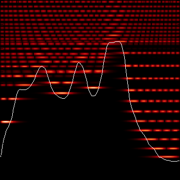
Das Bild zeigt die "lokale Zustandsdichte", also die Wahrscheinlichkeitsdichte der Energieeigenfunktionen, aufgetragen an den jeweiligen Energien (Energie vertikal, Ort horizontal).
Sehen Sie sich die Eigenfunktionen für Standard-Beispiele an (harmonischer Oszillator, Kasten, usw.): QM II: Lokale Zustandsdichte in Beispielen
Laden Sie den Quell-Code herunter: Yorick Quellcode Eigenfunktionen im Potentialgebirge
2013: Foundations of Quantum Mechanics
Lecture series by Florian Marquardt, summer term 2013
This lecture series addresses questions related to the foundations of Quantum Mechanics.
Overview
Have you ever wondered about the mysterious "collapse of the wave function" or the "wave-particle duality"? Does Schrödinger's cat make you uneasy? Do you have a feeling that there could be a deeper, more 'microscopic' theory underlying Quantum Mechanics? Do you believe that trajectories are ruled out by Quantum Mechanics? Are you confused by the concept of spin or by fermions vs. bosons? Do you want to learn how the founding fathers' "Gedankenexperiments" are now routinely realized in the labs?
This lecture series addresses questions related to the foundations of Quantum Mechanics. Topics will include:
- Bell's inequalities and Entanglement
- Measurements
- Decoherence and the quantum-to-classical crossover
- Interpretations of Quantum Mechanics (including Bohm's pilot wave and Nelson's Stochastic Quantization)
- Extensions of Quantum Mechanics (for example "spontaneous localization")
- Geometric phases (Aharonov-Bohm effect and all that)
- Particle statistics
- Quantum electrodynamics (including vacuum effects, renormalization, and Stochastic Electrodynamics)
- Relativistic quantum mechanics
The lectures require knowledge as obtained in a standard first course on Quantum Mechanics (more background will be beneficial but not absolutely needed). Master-level students and PhD students (as well as postdocs) will probably get the most out of this course.
Videos
The lectures are recorded on video and put online during the term as they become available. You can find them on the Erlangen server:
Schedule
There will be two 90-minute lectures per week plus one 90-minutes tutorial. Due to some travel-related absences of the lecturer during the term (as well as some public holidays), we will re-arrange the schedule and possibly skip some of the tutorials to keep the full 28 90-minutes lectures. We will arrange the full schedule in the first week.
We intend to record the lectures on video and post them online.
Times and rooms:
- Monday 15:15-16:45, lecture hall D
- Thursday 14:15-15:45, lecture hall D ( changed from earlier announcements)
- Friday 14:15-15:45, lecture hall F
Start: Monday, April 15, 15:15, lecture hall D.
Schedule (L=lecture, T=tutorial), subject to changes:
- April: 15-L, 18-T (17:15 in Hall E!), 19-L, 22-L, 25-L, 26-L, 29-L
- May: 2-T (17:15 in Hall E!), 3-T, 6-L, 10-L, 13-L, 16-T, 17-L, 23-L (changed to lecture; 17:15 in Hall E!), 24-T, 27-L, 31-L
- June: 3-L, 6-T (17:15 in Hall E!), 7-L, 10-L, 13-L, 14-L, 17-L, 20-T, 21-T, 24-L, 27-L, 28-L
- July: 1-T (changed to tutorial), 4-L, 5-L, 8-L, 11-T, 12-L, 15-L, 18-L, 19-L
Lecture Notes
- Lecture Notes Part 1 (PDF) (Introduction, Bell's inequalities and entanglement; Pages 1-46)
- Lecture Notes Part 2 (PDF) (Bell tests, entanglement, measurement; Pages 47-78)
- Lecture Notes Part 3 (PDF) (Weak measurements, decoherence; Pages 79-119)
- Lecture Notes Part 4 (PDF) (Interpretations of Quantum Mechanics, Extensions of Quantum Mechanics; Pages 120-168)
- Lecture Notes Part 5 (PDF) (Geometrical Phases, Particle Statistics, QED, Dirac Equation; Pages 169-231)
Original Literature
Note: Most of these papers are in German. English translations may be found in the book 'B. L. van der Waerden, editor, Sources of Quantum Mechanics (Dover Publications, 1968) ISBN 0-486-61881-1.
- On the Theory of Quanta, PhD thesis of Louis-Victor de Broglie (1924), English translation by A. Kracklauer: Download e-book
- Heisenberg's original matrix mechanics - This is the work that created the modern theory of quantum mechanics (Heisenberg 1925). Heisenberg wanted to tackle the question of how to predict correctly the intensities of atomic transition lines, as Bohr had already clarified how to obtain the transition frequencies. Heisenberg began by noticing that, according to Bohr, the correct quantum transition frequencies do not depend just on the current state of motion (as do the frequencies of emitted radiation for a classical orbit), but rather on two states (initial and final). Likewise, in classical theory, the intensities of emitted radiation would be given by the squares of the Fourier amplitudes of the oscillating dipole moment for a given orbit. In an ingenious step, Heisenberg then postulated that instead of a set of Fourier amplitudes for a given orbit (enumerated by one index), one would have to introduce a set of amplitudes depending on two indices, one for the initial, the other for the final state. He assumed that the equations of motion for those amplitudes looked formally the same as in classical theory (Heisenberg equations of motion). The last crucial ingredient is the commutation relation. This he derived by looking at the linear response of an electron to an external perturbation (essentially deriving something like Kubo's formula, containing the commutator) and then demanding that the short-time response would be always that of a free, classical electron. This fixes the commutator between position and momentum. Thus was born matrix mechanics. He applied this immediately to the harmonic oscillator and also dealt with the anharmonic oscillator using perturbation theory. See also Heisenberg's Nobel Lecture from 1933 to learn more about his view on these developments, and the slightly earlier overview (Heisenberg 1928 (Naturwissenschaften)) that also includes much of the developments before matrix mechanics.
- The formalism of matrix mechanics - The formalism of matrix mechanics was then developed fully by Born, Jordan and Heisenberg (Born, Jordan and Heisenberg 1926). They discuss: canonical transformations, perturbation theory, angular momentum, eigenvalues and eigenvectors. In addition to the formalism, that work also contains the earliest discussion of a quantum field theory: A linear chain of masses coupled by springs is quantized and solved by going over to normal modes. As a result, they find the Planck spectrum of thermal equilibrium, as a direct consequence of the newly developed quantum mechanics!
- The hydrogen atom in matrix mechanics - Wolfgang Pauli (Pauli 1926) managed to apply the new matrix mechanics to the hydrogen atom. He found the correct energy spectrum, as well as the correct Stark effect corrections to the energy in an applied electric field. In this solution, he makes use of the Runge-Lenz vector which is an additional conserved quantity known from classical mechanics for the Kepler problem, denoting the orientation of the elliptical orbit in space.
- The Schroedinger equation - Shortly after Heisenberg's work, Schroedinger came up with the equation that now carries his name. The essential idea was to start from the Hamilton-Jacobi equation, claim the action is the logarithm of some wave function psi (think WKB!), and derive a quadratic form of psi that is to be extremized (Schroedinger equation from the variatonal principle). This leads to the stationary Schroedinger equation, which he then solves for the hydrogen atom, as well as for the harmonic oscillator, the rotor and the nuclear motion of the di-atomic molecule (Schroedinger 1926a and Schroedinger 1926b).
- The probabilistic interpretation - While for a single electron inside an atom it might still be conceivable to view the wavefunction as some sort of smeared-out charge density, this view clearly becomes untenable when one moves to scattering processes, where the final scattered wave spreads out over a large region of space, whereas physically the particle will be detected at a point-like location. Thus it happened that during the investigation of quantum-mechanical scattering processes Max Born (Born 1926) was lead to the conclusion that the wave function has something to do with the probability of detecting a particle at some location. He at first incorrectly guessed the wave function itself gives the probability, but then inserted a famous footnote (on page 3 of this work) that says one should take the square! See also Max Born's Nobel lecture from 1954 for a discussion of the development of quantum mechanics.
- The uncertainty relation - Heisenberg showed that the precision with which position and momentum can be measured cannot be arbitrarily high for both these quantities simultaneously (Heisenberg 1927). This work contains also the discussion of the famous "Heisenberg microscope" gedankenexperiment, where one tries to determine the position of an electron only to find that by doing so one destroys any interference pattern that might have existed without this act of observation.
- Spin - The electron spin was introduced by Wolfgang Pauli (Pauli 1927) as an additional discrete degree of freedom that could take two values. (Note: The Pauli spin matrices make their first appearance on page 8 of this work)
2012/13: Quanten und Felder - Theoretische Physik für Materialphysiker (VL mit Übung)
Dozent: Prof. Dr. Florian Marquardt
Diese Vorlesung erklärt sowohl die Quantenmechanik als auch die Elektrodynamik. Sie ist geeignet für Materialphysik-Studenten, aber auch für Lehramtsstudenten.
- Ort und Zeit: Die Vorlesung findet statt am Dienstag, 10-12 (Hörsaal F) und Donnerstag, 10-12 (Hörsaal F). Beginn jeweils um 10:15.
- Die erste Vorlesung (mit Besprechung der Übungseinteilung) findet statt am Dienstag, 16.10.2012.
Klausur: Dienstag, 12. Februar, 10-12 Uhr, Hörsaal E
- Bitte kommen Sie schon kurz vor 10:00 in den Hörsaal, so dass wir rechtzeitig um 10:00 mit der Ausgabe der Blätter starten können
- Klausurumfang: 120 min
- Hilfsmittel: Ein handschriftlich, beidseitig beschriebenes DIN A4 Blatt als Formelsammlung (keine Kopie). Keine technischen Hilfsmittel (Taschenrechner, Handy, ..).
- Bringen Sie Ihren Ausweis sowie Ihren Studentenausweis zur Klausur mit
Klausureinsicht: Dienstag, 26. Februar 15-16 Uhr, SR 02.779
- Den Notenschlüssel der Klausur finden Sie hier (PDF)
Nachklausur: Donnerstag, 11. April 2013, 10-12 Uhr, Hörsaal D
- Bitte kommen Sie schon kurz vor 10:00 in den Hörsaal, so dass wir rechtzeitig um 10:00 mit der Ausgabe der Blätter starten können
- Klausurumfang: 120 min
- Hilfsmittel: Ein handschriftlich, beidseitig beschriebenes DIN A4 Blatt als Formelsammlung (keine Kopie). Keine technischen Hilfsmittel (Taschenrechner, Handy, ..).
- Bringen Sie Ihren Ausweis sowie Ihren Studentenausweis zur Klausur mit.
Nachklausur-Einsicht: Mittwoch, 24. April 16-17 Uhr, SR 02.779
Übungsblätter
- Blatt 1 (PDF)
- Blatt 2 (PDF)
- Blatt 3 (PDF)
- Blatt 4 (PDF)
- Blatt 5 (PDF)
- Blatt 6 (PDF)
- Blatt 7 (PDF)
- Blatt 8 (PDF)
- Blatt 9 (PDF)
- Blatt 10 (PDF)
- Blatt 11 (PDF)
- Blatt 12 (PDF)
- Blatt 13 (PDF)
- Blatt 14 (PDF)
Vorlesungsskript
Quantenmechanik:
- Skript Teil 1 (PDF)
- Skript Teil 2 (PDF) (Wellenpaket, Formalismus; Seiten 13-29)
- Skript Teil 3 (PDF) (Unschärferelation, Heisenbergbild; Zwei-Niveau-System, Harm. Oszillator; Seiten 30-48)
- Skript Teil 4 (PDF) (kohärente Zustände, Wasserstoff-Atom; Seiten 49-57)
- Skript Teil 5 (PDF) (Wasserstoff-Atom (Fortsetzung), Streuung, Störungsrechnung; Seiten 58-75)
- Skript Teil 6 (PDF) (Weitere Aspekte der Quantenmechanik (Magnetfeld, Spin, Viele Freiheitsgrade, Fermionen und Bosonen); Seiten 75-80)
Elektromagnetismus:
- Skript Teil 7 (PDF) (Felder, Maxwell-Gleichungen, Potentiale; Seiten 1-6)
- Skript Teil 8 (PDF) (Elektromagnetische Wellen, Energieerhaltung, Statische Phänomene; Seiten 7-19)
- Skript Teil 9 (PDF) (Dipol, Magnetostatik, Kapazitäten, Induktivität; Abstrahlung von Wellen; Seiten 20-38)
- Skript Teil 10 (PDF) (Polarisation, Maxwell-Gleichungen in Materie; Seiten 39-44)
- Skript Teil 11 (PDF) (Maxwell-Gleichungen in Materie (Fortsetzung), Randbedingungen, Wellen in Materie und an Grenzflächen; Seiten 45-56)
2012/13: Recent progress in cavity optomechanics
Lecturer: Prof. Dr. Florian Marquardt
This lecture gives insights into recent progress in an active research area dedicated to the interplay of nanomechanical motion and light (or electromagnetic radiation fields).
(2 hours / week, exercises discussed in class)
We are flexible with the schedule. We will meet for a first time on Tuesday, 16.10., at 16:00, in the small discussion room next to the office of Florian Marquardt, building B3, Staudtstr. (top floor).
Videos
Quantum Mechanics at the Macro-Scale (on Vimeo), brief lecture on the foundations of quantum mechanics, for a general audience. Lecture delivered by F. Marquardt at an interdisciplinary Kavli Frontiers of Science Symposium, Irvine (California), April 2011. This introduced subsequent lectures by Klaus Hornberger and Konrad Lehnert (also on Vimeo).
2012: Theoretische Physik 3 für Materialphysiker: Vielteilchenphänomene
Dozent: Prof. Dr. Florian Marquardt
Grundvorlesung im Bachelorstudium für Materialphysiker, 4. Semester (auch für Lehramtskandidaten)
- Zeit und Ort: Dienstag und Donnerstag, 10-12 Uhr, Hörsaal F
- Übungen: Donnerstag, 16-19 Uhr, SR 02.779 und Freitag, 16-19 Uhr, SR 02.779; Beginn der Übungen schon in der ersten Semesterwoche; Übungsblätter werden jeweils am Donnerstag ausgegeben (und die Lösungen eingesammelt). Die Übungen bestehen aus Präsenzübungen und Besprechung der Hausaufgaben.
- Übungsblätter:
- Siehe auch die thematisch verwandte Physik-Bachelor Vorlesung aus dem Winter 2010/11, mit einem Skript sowie Links zu Simulationsfilmen usw: Statistische Physik und Thermodynamik
Klausur: Dienstag, 24. Juli, 10-12 Uhr, Hörsaal D
- Bitte kommen Sie schon kurz vor 10:00 in den Hörsaal, so dass wir rechtzeitig um 10:00 mit der Ausgabe der Blätter starten können
- Klausurumfang: 120 min
- Hilfsmittel: Ein handschriftlich, beidseitig beschriebenes DIN A4 Blatt als Formelsammlung (keine Kopie). Keine technischen Hilfsmittel (Taschenrechner, Handy, ..).
- Bringen Sie Ihren Ausweis sowie Ihren Studentenausweis zur Klausur mit.
Klausureinsicht: Mittwoch, 08. August und Donnerstag, 09. August, 11-12 Uhr, 02.771
Nachklausur: Es wird mündliche Nachprüfungen von 45 Minuten Dauer geben, in der ersten Vorlesungswoche, vom 15.-19. Oktober 2012. Bitte vereinbaren Sie mindestens eine Woche vorher einen Termin mit Florian Marquardt.
2012: Moderne Quantenphysik (Scheinseminar zur theoretischen Physik)
Dozenten: Michael Thoss und Florian Marquardt
Zeit und Ort: Dienstags, 14-16 Uhr, Seminarraum S 02.779 (Aufgang B3)
Thematik: Die Quantenmechanik wird heutzutage erfolgreich angewendet auf die Beschreibung von natürlichen Systemen (wie Atomen und Molekülen), als auch auf die Analyse und das Design von künstlichen Systemen (wie elektronischen Schaltkreisen auf der Nanoskala). In diesem Seminar sollen zuerst einige allgemein anwendbare Methoden und Konzepte besprochen werden, die für die theoretische Beschreibung von Quantendynamik grundlegend sind. Es sollen dann weiterhin relevante moderne Anwendungen diskutiert werden.
Ablauf: Bitte melden Sie sich bei uns vor dem Start des Semesters per email, wenn Sie sich für eines der Themen entschieden haben, die unten aufgelistet und noch nicht vergeben sind. Wir werden Ihnen dann relevante Literatur nennen.
Bitte verwenden Sie StudOn zum Abruf aktueller Informationen über dieses Seminar!
Auf StudOn finden Sie diese Informationen unter
Um dort die Themen zu sehen, müssen Sie dem Kurs "beitreten".
Beim ersten Treffen werden wir noch einmal kurz die Thematik besprechen. Vor jedem Vortrag gibt es in der Woche zuvor einen Probevortrag, am Donnerstag, zwischen 16 und 19 Uhr. Die Vorträge selbst sollen auf ca. 60 Minuten angelegt sein, als Tafelvorträge (ggf. mit einigen Bildern per Beamer). Dazu kommt dann noch die Zeit für Fragen.
Themen:
Zeitabhängige Formulierung der Quantenmechanik, (getriebenes) Zweiniveausystem
Schwingungs-Wellenpaketdynamik im schwingenden Molekül
Wellenpaketdynamik, Rydberg-Atome
Zeitabhängige Schrödingergleichung: Numerische Simulation
Quanteninformationsverarbeitung
Cooper-Paar-Box als supraleitendes qubit
Adiabatische Dynamik und Berry-Phasen
Dichtematrix und Mastergleichung (dissipative Blochvektordynamik)
Rabi-Oszillationen in Atomen
Quantenelektrodynamik in supraleitenden Schaltkreisen (Jaynes-Cummins-Modell)
Messprozess
Wignerfunktionen und Vermessung von Quantenzuständen (Quantenoptik, Mikrowellenresonatoren)
Bose-Einstein-Kondensate
Kalten Atome in optischen Gittern
Nanomechanik und Optomechanik
EPR-Paradox und Bellsche Ungleichungen
2011/12: Theorie-Vertiefung 1 (Quantenmechanik II, Masterstudium)
Zeit und Ort: Montag und Mittwoch, 10-12, Hörsaal D
Übungen: Do 16-19
Klausur: Mittwoch, 8. Februar, 10-12, Hörsaal D
- Bitte kommen Sie um 09:50 Uhr in den Hörsaal, so dass wir rechtzeitig um 10:00 mit der Ausgabe der Blätter starten können
- Dauer der Klausur: 120 Minuten
- Hilfsmittel: Ein handschriftlich, beidseitig beschriebenes DIN A4 Blatt. Ansonsten sind keine weiteren Hilfsmittel zugelassen
- Bitte bringen Sie Ihren Personalausweis und Studentenausweis mit
Klausureinsicht: Dienstag, 21. Februar, 14 Uhr, SR 02.779
Nachklausur: Donnerstag, 12.4.2012, 10-12 Uhr, Hörsaal E
Seminar zu aktuellen Themen in der Optomechanik
Dozent: Prof. Dr. Florian Marquardt
Diskussion aktueller Literatur und Forschungsthemen
Zeit und Ort: 3-stündig, Ort und Zeit nach Vereinbarung; erste Besprechung: Mittwoch, 19.10., 15:15 in Raum 02.785
2011: Theoretische Physik 3 für Materialphysiker: Vielteilchenphänomene
Dozent: Prof. Dr. Florian Marquardt
Grundvorlesung im Bachelorstudium für Materialphysiker, 4. Semester
Zeit und Ort: Dienstag und Donnerstag, 10-12 Uhr, Hörsaal F; Übungen: Mittwoch, 16-19 Uhr, SR 02.779 und Donnerstag, 16-19 Uhr, SR 01.332; Beginn der Übungen in der zweiten Semesterwoche
Klausur: Dienstag, 2. August, 10-12, Hörsaal E
- Bitte kommen Sie schon kurz vor 10:00 in den Hörsaal, so dass wir rechtzeitig um 10:00 mit der Ausgabe der Blätter starten können
- Lehramtsstudenten und Materialphysiker schreiben dieselbe Klausur für 10 ECTS-Credits
- Klausurumfang: 120 min, 4 Aufgaben
- Hilfsmittel: Ein handschriftlich, beidseitig beschriebenes DIN A4 Blatt als Formelsammlung (keine Kopie). Keine technischen Hilfsmittel (Taschenrechner, Handy, ..).
- Bringen Sie Ihren Ausweis sowie Ihren Studentenausweis zur Klausur mit.
- Die Klausur ist korrigiert und die Noten dem Prüfungsamt übermittelt und ab Do. 04.08 über mein Campus einsehbar. Falls Sie Ihre Ergebnisse nicht über mein Campus einsehen können oder Sie sonst Einsicht in Ihre Klausurkorrektur wollen, kommen Sie bitte zwischen 11.00 und 12.00 am Fr. 05.08 oder Mi. 10.08 zur Klausureinsicht ins Zimmer 02.771.
Nachklausur: Dienstag, 11. Oktober, 10-12, Hörsaal E
Übungsblätter:
2010/11: Statistische Physik und Thermodynamik
Dozent: Prof. Dr. Florian Marquardt
Grundvorlesung im Bachelorstudium, 5. Semester
Zeit und Ort: Dienstag und Donnerstag, 10-12 Uhr, Hörsaal E, Übungen freitags, 13-16 Uhr, Beginn am Dienstag, 19. Oktober, 10:15
Klausur: Dienstag, 8. Februar, 10-12, Hörsaal E; Nachholklausur: Donnerstag, 28. April, 10-12, Hörsaal E
Aufzeichnungen: Die Vorlesungen werden vom Rechenzentrum auf Video aufgezeichnet und verfügbar gemacht.
- Link zu den Video-Aufzeichnungen (auch auf iTunes University / Naturwissenschaften)
Klausurbedingungen
- Bitte kommen Sie schon kurz vor 10:00 in den Hörsaal, so dass wir rechtzeitig um 10:00 mit der Ausgabe der Blätter starten können
- Bachelorklausur: 120 min, 4 Aufgaben
- Lehramtsklausur: 100 min, 3 Aufgaben
- Lehramtsstudenten können auch die Bachelorklausur schreiben, wenn sie die vollen ECTS-Credits bekommen wollen. Sie müssen dies allerdings vor Beginn der Klausur entscheiden.
- Hilfsmittel: Ein handschriftlich, beidseitig beschriebenes DIN A4 Blatt als Formelsammlung (keine Kopie). Keine technischen Hilfsmittel (Taschenrechner, Handy, ..).
- Bringen Sie Ihren Ausweis sowie Ihren Studentenausweis zur Klausur mit.
- Die Musterlösung der Klausur wird am Do., 10.2., in der Vorlesung vorgerechnet.
- Klausureinsicht und Fragen zur Korrektur am Do. 17.02.2011, Raum 02.779, 10-12 Uhr.
- Wenn Sie nicht zur Klausur als Erstversuch antreten wollen, können Sie zurück treten (bitte fairerweise vorher eine email an Björn Kubala senden), und wir werden "nicht erschienen" in MeinCampus eintragen. Das hat die Auswirkung, dass erst die Nachholklausur als Erstversuch gewertet wird. Wir empfehlen allerdings im Regelfall, schon die Klausur als Erstversuch zu belegen.
Überblick Klausurergebnisse
- Klausurergebnisse sind über mein Campus einsehbar. (Diplom)studenten, deren Noten nicht über mein Campus verwaltet werden, können sich ihre Ergebnisse (und gegebenenfalls einen Schein) im Zimmer 02.771 abholen.
- Histogramm der Punkteverteilung (PDF)
Nachklausur
- Die Nachklausur ist korrigiert. Klausurergebnisse sind ab Montag über mein Campus einsehbar. (Diplom)studenten, deren Noten nicht über mein Campus verwaltet werden, können sich ihre Ergebnisse (und gegebenenfalls einen Schein) im Zimmer 02.771 abholen.
- Klausureinsicht und Fragen zur Korrektur am Mo. 09.05.2011, Raum 02.779, 12-14 Uhr.
Klausuranmeldung
Hier eine Information von Frau Forkel zur Anmeldung bei Mathematikern:
"Die Pruefungsnummer fuer die Mathestudenten mit Nebenfach theoretische Physik ist 62401 und die Bachelorstudenten muessten sich dafuer ueber mein Campus auch problemlos anmelden koennen. Sollte es Schwierigkeiten mit der Anmeldung geben, verweisen Sie die Studenten doch bitte direkt an mich.
Die Masterstudenten koennen sich aus technischen Gruenden nicht ueber mein Campus anmelden. Fuer diesen Personenkreis bitten wir Sie, die Leistung bei der Notenverbuchung unter derselben Pruefungsnummer mit zu erfassen."
Kurze Inhaltsangabe:
- Boltzmann-Gibbs-Verteilung, d.h. kanonische Verteilung (klassisch und quantenmechanisch, Zustandssumme, freie Energie und Entropie, einfache Argumente für die Boltzmannverteilung)
- Einfache Anwendungen in der Quantenmechanik (Zweiniveausystem, harmonischer Oszillator, Wärmestrahlung)
- Minimalprinzip der freien Energie, Druck und chemisches Potential
- Freie Quantengase (Fermigas, Bosegas, klassisches ideales Gas als Grenzfall)
- Wechselwirkung und Phasenübergänge (Ising-Modell, Molekularfeldnäherung, Langreichweitige Ordnung und Ordnungsparameter, Exakte Resultate, Kritische Phänomene, Fluktuationen, Renormierungsgruppe)
- Thermodynamik (Thermodynamische Potentiale, Phasendiagramme, Kreisprozesse)
- Ausblick: Kinetische Gleichung, Hydrodynamik, Fluktuationen und Dissipation, Thermalisierung
Aufzeichnungen:
Die Vorlesungen werden vom Rechenzentrum auf Video aufgezeichnet und verfügbar gemacht.
- Link zu den Video-Aufzeichnungen (auch auf iTunes University / Naturwissenschaften)
Skript:
Eine noch unkorrigierte Version des Skriptes mit den Kapiteln 1-9 finden Sie hier:
Vorlesungsumfrage:
- Offizielle Ergebnisse der Umfrage (pdf) (Übung: Der Mittelwert zur 'Vorlesung im Allgemeinen', und damit auch der Globalindikator, ist irreführend. Erkennen Sie, warum?)
- Statistische Physik Vorlesungsumfrage 2011 Kommentare (meine Antworten auf ein paar Kritikpunkte)
Fragen und Antworten:
Häufig gestellte Fragen und Missverständnisse, Hinweise und Tricks
Vorlesungen (Stichpunkte, Materialien):
- 1 - (Di., 19.10.2010) Kapitel 1: Einleitung, Wo ist Statistische Physik und Thermodynamik wichtig?, Computersimulationen: Heuristische Beobachtung der Relaxation ins Gleichgewicht, Maxwell-Boltzmann-Verteilung, Definition der Temperatur über die kinetische Energie, Ortsverteilung, Effekte der Wechselwirkung; siehe
Filme zur Relaxation ins Gleichgewicht: - Relaxation ins Gleichgewicht aus beliebiger Anfangsverteilung: Media:RelaxFortyTwo.mov
- Geschwindigkeitsverteilung instantan: Media:MaxwellBoltzmannInstantaneous.mov
- Maxwell-Boltzmann Geschwindigkeitsverteilung, zeitgemittelte Dichte: Media:MBdensity.mov
- Verteilung für leichte und schwere Teilchen (blaue Teilchen sind 16 mal schwerer, ihre Geschwindigkeitsverteilung ist rechts oben abgebildet): Media:MBtwoSpecies.mov
- Verteilung im Ort für Potentiallandschaft. Rechts oben befindet sich eine attraktive Potentialmulde, links unten ein repulsiver Potentialberg: Media:BoltzmannForPotential.mov
- Verteilung im Ort im selben Potential, aber für abgekühlte Teilchen (blauer Punkt links oben zeigt künstliche Reibung an), Effekte der Wechselwirkung: Media:BoltzmannDrop.mov
Diese Simulationen wurden in der Public-Domain Interpretersprache Yorick geschrieben, die besonders für numerische Anwendungen und schnelle grafische Darstellung von Simulationsergebnissen geeignet ist. Die resultierenden Bildersequenzen wurden dann mit Hilfe von FrameByFrame in QuickTime Movies konvertiert. Beispiele für den Quellcode, ohne Kommentare und mit überflüssigen Code-Teilen: Beliebige Anfangsverteilung (Media:particlegasRelax.i), Instantane Geschwindigkeitsverteilung (Media:particleGasMB.i), MB-Verteilungsdichte (Media:particleGasMB2.i), Leicht/Schwer (Media:particlegasMB2twospecies.i), Verteilung im Ort (Media:particlegasPotential2.i), und Verteilung im Ort mit Abkühlung (Media:particlegasPotential2Cool.i).
- 2 - (Do., 21.10.) Anmerkungen zur Verteilung im Konfigurationsraum, Konzept des Teilsystems eingebettet in ein Gesamtsystem oder Wärmebad, siehe Filme zum Konzept des Teilsystems, eingebettet in ein Wärmebad oder ein größeres Gesamtsystem:
- Wechselwirkend (blaue) Teilchen inmitten eines Gases kleiner Teilchen (gelb): Media:HeatBathFewBigParticles.mov
- Dasselbe, aber schneller. Zwischen den Teilchen wirkt eine attraktive langreichweitige Kraft: Media:HeatBathFastForward.mov
- Ausschnitt eines Kristallgitters (die blauen Atome sind identisch mit dem Rest, bilden aber das gedachte Teilsystem). Man beachte, wie die anfängliche kollektive Schwingung bald in unregelmässige Wärmebewegung des Kristallgitters übergeht: Media:CrystalLatticeWobbly.mov
- Folien dazu: Media:HeatBathSlides.pdf
- Heuristische Einführung der quantenmechanischen Verteilung, Inhaltsangabe der Vorlesung, Kapitel 2: Kanonische Verteilung, Zustandssumme, Mittelwerte, Energie als Funktion der Temperatur, Wärmekapazität, Energiefluktuationen, Zusammenhang zwischen beiden
- 3 - (Di., 26.10.) Freie Energie, Entropie aus der freien Energie und aus den Wahrscheinlichkeiten, Zusammengesetzte unabhängige Systeme: Faktorisierung der Wahrscheinlichkeit und der Zustandssumme, Additivität und Extensivität von F, E, S, Die Zustandsdichte
- 4 - (Do., 28.10.) Wahrscheinlichkeitsdichte der Energie und Zustandsdichte in einem grossen System, Kapitel 3: Einfache Ableitungen der kanonischen Verteilung, 3.1: Ableitung aus der mikrokanonischen Verteilung, Film (Media:BoltzmannLattice.mov) zur Boltzmannverteilung eines Teilsystems ausgehend von Gleichverteilung aller Konfigurationen mit derselben Energie im Gesamtsystem (die Radien der Kreise geben die Energie an, die Verteilung eines Teilsystems ist links unten gezeigt), 3.2: Ableitung aus Additivität und Unabhängigkeit, 3.3: Ableitung aus der Maximierung der Entropie unter Nebenbedingungen, Kapitel 4: Einfache Anwendungen der kanonischen Verteilung, 4.1: Das Zweiniveausystem [Hinweis: In der Erklärung zur geometrischen Idee hinter den Lagrange-Multiplikatoren sollte es heissen, dass die Gradienten parallel sind (nicht gleich), und der Faktor zwischen ihnen ist der Lagrange-Multiplikator.]
- 5 - (Di., 2.11.) Freie Energie und Entropie für das Zweiniveausystem, Spin im Magnetfeld, magnetische Suszeptibilität, Curie-Gesetz, Allgemein: Suszeptibilität und Fluktuationen, 4.2: Der harmonische Oszillator, Bose-Verteilung für die mittlere Besetzungszahl
- 6 - (Do., 4.11.) Klassischer Gleichverteilungssatz für die mittlere Energie eines harmonischen Oszillators, Wärmekapazität, Freie Energie und Entropie, 4.3: Gitterschwingungen und Wärmestrahlung, Darstellung durch Normalmoden ergibt viele unabhängige harmonische Oszillatoren, Zustandsdichte der Feldmoden, k-Raum
- 7 - (Di., 9.11.) Relaxation ins Gleichgewicht für ein Wellenfeld mit nichtlinearem Term (siehe Filme für lineares Wellenfeld Media:LinearWaveField.mov und Relaxation im nichtlinearen Feld Media:NonlinearWaveField.mov, auch zu späten Zeiten Media:NonlinearWaveFieldLateTimes.mov; rechts oben ist die Verteilung der Energie im k-Raum gezeigt), Berechnung der Gesamtenergie des Feldes im thermischen Gleichgewicht, Stefan-Boltzmann-Gesetz, Abstrahlung, Wärmekapazität für die Gitterschwingungen, Plancksches Strahlungsgesetz, Kapitel 5: Klassischer Limes, neue Basis im Phasenraum, Zustandssumme durch Integral im Phasenraum genähert, thermische de Broglie Wellenlänge
- 8 - (Do., 11.11.) Kapitel 6: Makroskopische Variablen, Druck, chemisches Potential, 6.1: Minimierung der freien Energie und Aus-Integration von Variablen, partielle Zustandssumme Z(x) und freie Energie F(x), Beispiel: Auftreib beim "Ballon" (siehe Film Media:Balloon.mov), 6.2 Der Druck, Gleichgewichtsposition einer Trennwand zwischen zwei Gasen, Beweise thermodynamische Definition des Druckes stimmt mit der mechanischen überein, Fluktuationen eines Volumens bestimmt durch Kompressibilität, 6.3: Das chemische Potential, freie Energie abhängig von fluktuierender Teilchenzahl im Teilvolumen F(N1), chemisches Potential überall gleich im Gleichgewicht
- 9 - (Di., 16.11.) Anwendung des chemischen Potentials auf inhomogene Systeme, Teilchenzahlfluktuationen, 6.4 Die großkanonische Verteilung, großkanonische Zustandssumme und großkanonisches Potential, Kapitel 7: Gase, 7.1 Identische Teilchen: Fermionen und Bosonen
- 10 - (Do., 18.11.) Vielteilchenbasiszustände, Besetzungszahldarstellung, für Bosonen und Fermionen, Erwartungswerte von Einteilchenoperatoren, 7.2 Das Fermigas, Fermi-Dirac Verteilung, Zustandsdichte von Teilchen mit Masse in 1D, 2D, 3D, Metall vs. Halbleiter
- 11 - (Di., 23.11.) Energie und Wärmekapazität des Fermigases bei tiefen Temperaturen, zuerst bei konstanter Zustandsdichte, dann Sommerfeldentwicklung für beliebige Zustandsdichte, Entartungsdruck bei T=0, Allgemeiner Zusammenhang zwischen Zustandsgleichung pV und dem großkanonischen Potential, Allgemeine Formeln für Druck und chemisches Potential in dimensionsloser Notation für Teilchen in 3D, Entwicklungen für kleine Dichte (hohe Temperaturen) und hohe Dichte (kleine Temperaturen), Fluktuationen der Teilchenzahl
- 12 - (Do., 25.11.) Entropie des Fermigases, 7.3: Das Bosegas, Bose-Einstein-Verteilung, Bose-Einstein-Kondensation: makroskopische Besetzung des Einteilchen-Grundzustandes, Übergangstemperatur, Experimente an kalten Atomen, Wärmekapazität und Druck im idealen Bosegas als Funktion der Temperatur bzw. Dichte, Gross-Pitaevskii-Gleichung für die Dynamik des Bosekondensates, Superfluidität
- 13 - (Di., 30.11.) Nochmal Bemerkungen zur Superfluidität, mit Simulationen: Zeitentwicklung der Kondensatdichte (also |phi|^2), wenn sich ein Objekt hindurchbewegt: Ausstrahlung von Schallwellen, wenn es schneller ist als die Schallgeschwindigkeit im Kondensat (Film:Media:BECmotionFast.mov) und kein Energieverlust, wenn es langsamer ist (Film:Media:BECmotionSlow.mov) ; 7.4: Das klassische ideale Gas, als Grenzfall aus der Fermi- und Boseverteilung, Maxwell-Boltzmann-Verteilung, Zustandsgleichung, chemisches Potential und der quantenmechanische Anteil darin, freie Energie, Entropie, Energie des idealen Gases, alternative Herleitung aus der klassischen Zustandssumme; 7.5: Das reale Gas - Virialentwicklung, Idee der Clusterentwicklung in der Zustandssumme, Endresultat, Prinzip der graphischen Darstellung von Termen in der Störungsrechnung mit Diagrammen
- 14 - (Do., 2.12.) Kapitel 8: Phasenübergänge, Allgemeine Einleitung, 8.1 Das Ising-Modell, Spins auf Gitter und Energie einer Konfiguration, Computer-Experiment: Erzeugung typischer Konfigurationen in einer Monte-Carlo-Simulation, Beobachtung des Übergangs zur magnetischen Ordnung (Filme: Media:IsingMCblackAndWhite.mov und Media:IsingMCselectionFromSweep.mov; Hinweise: In beiden Filmen wird während der Simulation die Temperatur abgesenkt und man erkennt den Phasenübergang an der Bildung immer größerer Domänen; im zweiten Film ist zur besseren Veranschaulichung über benachbarte Spins gemittelt, so dass nur die großen Domänen völlig weiß oder schwarz erscheinen; Es wird der über das ganze Gitter gemittelte Spin als Funktion der Temperatur aufgetragen, wobei die vertikalen Skalenstriche den Temperaturen 1.5,1.6,...,2.8 entsprechen; die exakte Phasenübergangstemperatur liegt bei 2.269 in diesen Einheiten; zur Beschleunigung werden nur Ausschnitte aus dem gesamten Simulationslauf gezeigt), 8.2 Monte-Carlo Simulationen, Zufallspfad im Konfigurationsraum und kanonische Verteilung als stationäre Verteilung, Metropolis--Algorithmus
- 15 - (Di., 7.12.) 8.3 Molekularfeld-Näherung ("mean-field"), Selbstkonsistenzgleichung für räumlich gemittelte Magnetisierung, 8.4 Fluktuationen, Korrelationsfunktion, Suszeptibilität - Heuristische Diskussion der Korrelationsfunktion zweier Spins, langreichweitige Ordnung, Zusammenhang zwischen Fluktuationen der Magnetisierung und der Korrelationsfunktion
- 16 - (Do., 9.12.) Suszeptibilität und Beziehung zu den Fluktuationen der Magnetisierung, Auswertung in der Molekularfeld-Näherung, Curie-Weiss-Gesetz, Divergenz der Suszeptibilität an der kritischen Temperatur, 8.5 Exakte Lösung des 1D Ising-Modells, Zustandssumme als Spur über ein Produkt von Transfermatrizen
- 17 - (Di., 14.12.) Berechnung der Eigenwerte der Transfermatrix, Diskussion der Zustandssumme für hohe und tiefe Temperaturen, Rechnung inklusive Magnetfeld, kein Phasenübergang, aber sehr starkes Anwachsen der Suszeptibilität bei tiefen Temperaturen, Entropie-Argument für die Abwesenheit des Phasenüberganges in einer Dimension
- 18 - (Do., 16.12.) Unterschied zwischen den Dimensionen, Berechnung der Korrelationsfunktion im 1D Ising-Modell, Korrelationslänge divergiert für T gegen 0, 8.6 Exakte Lösung des 2D Ising-Modells, Ansatz wieder mit Transfermatrizen, Berechnung des größten Eigenwertes nötig, Endergebnis für die spontane Magnetisierung, Existenz eines Phasenüberganges, Vergleich mit Molekularfeld-Näherung: anderer kritischer Exponent, Wärmekapazität divergiert logarithmisch, 8.7: Freie Energie als Funktion der Magnetisierung, Landau-Theorie, Definition der magnetisierungsabhängigen freien Energie, Heuristische Erwartung, Computer-Experiment mit Auswertung aller Konfigurationen in einem 4x4-Gitter (Folien:Media:IsingKonfigurationen.pdf), Übergang von einem Minimum zu zwei Minima, Landau-Theorie als Taylorentwicklung in der Magnetisierung und in der Distanz zum kritischen Punkt, Landau-Theorie reproduziert mean-field Resultat
- 19 - (Di., 21.12.) Räumliche Mittelung über endliche Bereiche, Ordnungsparameterfeld, (siehe Folien: Media:IsingRGslides.pdf), Ginzburg-Landau-Theorie, Antwort auf ein lokales Magnetfeld, Korrelationsfunktion hat keine Skala bei T=T_c, 8.8 Universalität und Selbstähnlichkeit, kritische Exponenten für die Magnetisierung im Ising-Modell, Abhängigkeit von Raumdimension und Art des Ordnungsparameters, aber nicht von anderen mikroskopischen Details, flüssig-Gas kritischer Punkt liegt in der "Universalitätsklasse" des 3D Ising-Modells, Selbstähnlichkeit (fraktale Struktur) auf Skalen unterhalb der Korrelationslänge (siehe Film: Media:ZoomOutFractalField.mov), 8.9 Renormierungsgruppe, Idee der schrittweisen Vergröberung der Skala, Beispiel des 1D Ising-Modells, Elimination jedes zweiten Spins erzeugt effektives neues Modell mit renormierten Parametern, effektive Kopplung geht gegen Null wenn Anzahl der eliminierten Spins der Korrelationslänge entspricht (siehe Folien von oben).
- 20 - (Do., 23.12.) Renormierungsgruppe in 2D, Problem der neu generierten Kopplungen, RG-Fluss, Wilsons RG für das Ising-Modell in d Dimensionen, Ausintegrieren und reskalieren, Wilsons Flussgleichungen, (Film:Media:WilsonsRGFlow.mov)
- 21 - (Di., 11.1.) 8.10 Zerstörung langreichweitiger Ordnung durch thermische Fluktuationen, diskreter Ordnungsparameter vs. kontinuierliche Symmetrie, Fluktuationen in der 1D Kette zerstören langreichweitige Ordnung, Rechnung mittels Normalmodenzerlegung (Schallwellen), langreichweitige Ordnung vorhanden in 3D aber nicht in 2D, allgemeines Mermin-Wagner-Hohenberg-Theorem
- 22 - (Do., 13.1.) Kapitel 9. Thermodynamik, 9.1 Arbeit, Wärme, und der Zusammenhang zur Entropie; Adiabatische Kompression eines Gases (Film:Media:Compression.mov, Folien:Media:SlidesAdiabaticCompression.pdf), Isotherme Kompression, Wärme und Entropieänderung, Reversible vs. irreversible Prozesse, 9.2 Gesetze der Thermodynamik, Begriffe, Erster Hauptsatz (Energieerhaltung), Zweiter Hauptsatz (Richtung der Prozesse)
- 23 - (Di., 18.1.) Zweiter Hauptsatz nach Kelvin vs. Version von Claudius, Äquivalenz der Versionen, 9.3 Kreisprozess, Carnot-Prozess als reversibler Kreisprozess zwischen zwei Reservoiren, Definition des Wirkungsgrades, Prinzip der Wärmepumpe, Carnot-Prozess hat maximalen Wirkungsgrad, 9.4 Konstruktion der Thermodynamik aus den Hauptsätzen, Kein Prozess zwischen zwei Reservoiren ist effizienter als Carnot
- 24 - (Do., 20.1.) Definition einer absoluten Temperaturskala aus dem Carnot-Wirkungsgrad [Bem.: Es hätte darauf hingewiesen werden sollen, dass die Hintereinanderschaltung zweier Carnot-Prozesse wieder einen Carnot-Prozess ergibt, und deshalb die bei dieser Hintereinanderschaltung ins unterste Reservoir abgegebene Wärme gleich der für den direkten Prozess ist.], Satz von Clausius über zyklische Prozesse, Definition der Entropie, Entropie eines thermisch isolierten Systems nimmt niemals ab, 9.5 Die thermodynamischen Potentiale: Innere Energie [Bem.: C_p wurde falsch angeschrieben, es muss heissen C_p=(dQ/dT)_p=(dH/dT)_p mit H=E+pV], Freie Energie, Enthalpie, Gibbssche freie Energie, Großkanonisches Potential, Abnahme der freien Energie ergibt maximale beim isothermen Prozess verrichtete Arbeit, im Gleichgewicht eines isothermen Systems (bei festem Volumen) wird die freie Energie minimiert.
- 25 - (Di., 25.1.) Minimierung der Gibbsschen freien Energie bei konstanter Temperatur und konstantem Druck, Partielle Ableitungen und Funktionaldeterminante, Maxwell-Relationen, Stabilitätsbedingungen, 9.6 Thermodynamik der Phasenübergänge, pV-Diagramm und Koexistenzbereich für flüssig-gasförmig Übergang, Dichten sind jeweils konstant im Koexistenzbereich, latente Wärme aus der Entropieänderung, Bedingungen für das Phasengleichgewicht: Gleicher Druck und gleiches chemisches Potential in beiden Phasen, Phasengrenze im pT-Diagramm, Satz von Clausius-Clapeyron zur Temperaturabhängigkeit des Dampfdruckes
- 26 - (Do., 27.1.) 1. Ordnung vs. 2. Ordnung Phasenübergang (diskontinuierlich vs. kontinuierlich), Vergleich flüssig/gas mit magnetischem Übergang, Potential als Funktion der Dichte, Sprung in der Magnetisierung bzw. der Dichte, Phasendiagramme in der Ebene Magnetfeld/Temperatur bzw. chemisches Potential (oder Druck) vs. Temperatur, kein kritischer Punkt bei Übergang zum festen Kristall, da dort qualitative Änderung der Symmetrie, generisches Phasendiagramm fest/flüssig/gasförmig, Metastabile Zustände (überhitzte Flüssigkeit, übersättigter Dampf), Phänomenologische Van-der-Waals Zustandsgleichung
- 27 - (Di., 1.2.) 9.7 Der "dritte Hauptsatz"; 10. Kapitel: Fluktuationen und Nichtgleichgewicht, 10.1 Lineare Antwort und zeitabhängige Fluktuationen, Beispiel harmonischer Oszillator im Wärmebad, thermische Fluktuationen (Fillm:Media:OscillatorFluctuations.mov), lineare Antwort auf externen Kraftpuls (Film:Media:OscillatorLinearResponse.mov), Suszeptibilität, Oszillierende Kraft, frequenzabhängige Antwort, Fluktuationen charakterisiert durch Korrelator, Spektrum der Fluktuationen, Fluktuations-Dissipations-Theorem, klassische und quantenmechanische Variante, 10.2 Die Dichtematrix, Definition, Zeitabhängigkeit, Eigenschaften, Kubo-Formel für die lineare Antwort
- 28 - (Do., 3.2.) 10.3 Diffusion, Zufallspfad und Diffusionsgleichung, Drift bei externer Kraft, Boltzmannverteilung als Resultat im stationären Zustand, Einstein-Relation zwischen Mobilität und Diffusionskonstante, 10.4 Boltzmanns kinetische Gleichung, Verteilung im Impulsraum, Stöße (Film: Media:MaxwellBoltzmannInstantaneous.mov), Boltzmanngleichung, Beweis von Boltzmanns H-Theorem, Drift-Terme für inhomogene Situationen, 10.5 Hydrodynamische Gleichungen, Annahme des lokalen Gleichgewichts, Felder Massendichte, Strömungsgeschwindigkeit, Temperatur, qualitative Diskussion der Effekte, Navier-Stokes-Gleichung, Massenerhaltung, Energieerhaltung, Wärmeleitung und Reibungswärme, Abschluss der Vorlesung: Zurück zum Beispiel der Heliumwolke, Statistische Physik und Thermodynamik sind nützlich für Materialphysik, Nanophysik, Biophysik, Quantenoptik, Astrophysik, Kosmologie, und viele andere Bereiche in der Forschung.
Literatur:
Die Vorlesung selbst folgt keinem Buch, und es wird zuallererst der aufmerksame Besuch der Vorlesung, das Mitschreiben derselben, sowie die eigenständige Bearbeitung aller Übungsaufgaben empfohlen! Zum Nachlesen jedoch sind folgende Bücher neben vielen anderen geeignet:
- Schwabl, "Statistische Mechanik" --- Standardlehrbuch
- Nolting, "Grundkurs Theoretische Physik: Statistische Physik" --- Standardlehrbuch
- Becker, "Theorie der Wärme" --- Alt, aber sehr gut, mit vielen realistischen Beispielanwendungen
- Landau/Lifschitz, "Statistische Physik I" --- für Fortgeschrittene
- Huang, "Statistical Mechanics" --- Mein Lieblingsbuch zur Statistischen Physik. Besonders gute Abschnitte über Kinetik (Boltzmanngleichung) und kritische Phänomene
- Kadanoff, "Statistical Physics: Statics, Dynamics and Renormalization" --- Originelle Darstellung für Fortgeschrittene, Einführung in die Renormierungsgruppe, Original-Forschungsarbeiten, leider manche Tippfehler
Interessante Links zu thematisch relevanten Webseiten:
- Entweichen von Gasen aus Planetenatmosphären ("Atmospheric Retention lab") - illustriert die Bedeutung der Maxwell-Boltzmann Verteilung für die Entweichwahrscheinlichkeit. Im thermischen Gleichgewicht gibt es keine Planetenatmosphäre, weil sich jedes Gas über das ganze Weltall ausdehnen, d.h. entweichen würde. Allerdings sind die Zeitskalen für schwerere Moleküle (bzw. bei tieferen Temperaturen oder massiveren Planeten) sehr lang.
- Ising Modell Simulation - Monte-Carlo Simulation des Isingmodells in zwei Dimensionen, mit einstellbarer Temperatur und einstellbarem Magnetfeld. Der Prototyp für Phasenübergänge.
Übungen:
Übungsblätter und aktuelle Informationen finden sie hier.
2010: Quantum-optical phenomena in nanophysics
Lecture by Florian Marquardt (lecture delivered in English). Official German title was "Quantenoptische Phänomene in der Nanophysik"
About these lectures
Lectures by Florian Marquardt (summer term 2010)
These lectures deal with the modern topic of quantum optical phenomena in nanophysics. During the past decade, a variety of solid state nanosystems have been realized which can be described using the concepts of quantum optics.
The two main topics I discuss are quantum electrodynamics in superconducting circuits of microwave resonators and qubits ("circuit cavity QED") and nanomechanical resonators interacting with light ("optomechanics"), along with smaller sections on excitons in quantum dots and nitrogen vacancy centres in diamond. In addition, there are a number of general theory chapters (marked by a T in the chapter headings). These deal with concepts of general applicability, e.g. the quantum states of a field mode (coherent states, squeezed states, Wigner density), general two-level dynamics, the Jaynes-Cummings model, noise spectra, dissipation, decoherence, and Lindblad master equations. Since most of these general concepts are naturally introduced during the first chapter on circuit QED, that chapter might seem longer than it actually is.
This course may also complement nicely a traditional quantum optics course (geared towards free optical photons and atomic physics). For example, I go through the quantization of the electromagnetic field in some detail, but for the superconducting microwave resonator on a chip, instead of the field in free space. Students might be interested to see how much overlap there is, and that the concepts learned in one domain can be immediately applied in the other domain. On the other hand, it has to be admitted that this section on field quantization is the lengthiest technical part, and it may be skipped without problems.
Who will benefit from this course? I have tried to keep the discussion self-contained, so anyone with a first course in quantum mechanics should be able to follow. Thus, the lectures are already useful to third year students, but should be especially valuable to beginning PhD students who want to work on a topic at the intersection of nanophysics and quantum optics, or even on a more "traditional" quantum optics or atomic physics project. Most of the topics are taught at a level that the tools acquired can be immediately applied in practice. Only for some of the last lectures have I chosen an "overview" style, because by that time the students have already learned how it would work in detail.
Florian Marquardt (July 25, 2010)
Brief contents
- Lecture 1 1. Introduction: From ensembles to individual quantum systems, artificial quantum systems in nanophysics, field-matter interaction is based on oscillators (field) and two-level systems (atoms) T1. Basics of the harmonic oscillator: ladder operators, coherent states, coupling two oscillators, rotating wave approximation
- Lecture 2 (T1, continued) many coupled oscillators and normal modes, T2. Basics of the two-level system: Pauli matrices, Bloch vector, free precession, avoided crossing in the energy spectrum, time-dependent driving (Rabi-oscillations)
- Lecture 3 2. Quantum electrodynamics in superconducting circuits 2.1 Some basics about superconductivity: zero resistance, Meissner-Ochsenfeld effect, critical magnetic field, Cooper pairs, the BCS gap 2.2 The Cooper pair box: tunneling between two islands, the charging energy, the tunneling term, external control via a gate charge [erratum: near the end of the lecture, the arrow for the dipole moment of the Cooper pair box was drawn in the wrong direction. It should point from the negative to the positive charge, as always.]
- Lecture 4 (2.2 continued) Energy level spectrum of the Cooper pair box, approximation as a two-level system 2.3 The microwave transmission line resonator: Cavities (optical, 3D microwave), waveguides, transmission lines, discretized circuit description of a transmission line, LC oscillator, wave equation, passage to continuum limit
- Lecture 5 (2.3 continued) Overview: how to quantize the transmission line resonator, goal: Jaynes-Cummings model. Lagrangian and Hamiltonian description needed as steps towards quantum theory. Example: Simple LC oscillator, using flux as a variable. Lagrangian density for the transmission line. Quantizing the LC oscillator.
- Lecture 6 (2.3 continued) Quantizing the transmission line with periodic boundary conditions. Quantizing the transmission line resonator. Coupling to a Cooper-pair box.
- Lecture 7 2.4 The Jaynes-Cummings model: Examples: different microscopic physical models all lead to the JC model; e.g. optical cavity and atom, photonic crystal cavity and exciton, or vibrations in a lattice and a defect two-state system. T3. The JC model: Solution: Level scheme. Rotating-wave approximation. Resonant case and vacuum Rabi oscillations.
- Lecture 8 Continued Jaynes-Cummings model. 2.5 Jaynes-Cummings model in circuit QED. Transmission spectroscopy and avoided crossing in the strong coupling regime. Dispersive regime for non-destructive qubit readout.
- Lecture 9 T4. Dissipation in quantum systems. Relaxation. Density matrix. Lindblad Markoff master equations. Application to relaxation in a two-level system. Application to harmonic oscillator.
- Lecture 10 (continued with Lindblad equations) Application to harmonic oscillator. Pure dephasing. Bloch equations for a dissipative two-level system. T1 and T2 times. Expression of decay rates via quantum noise spectra. Some comments on the general structure of Lindblad master equations, especially for numerical solutions.
- Lecture 11 More detailed derivation of Fermi Golden Rule rates expressed via quantum noise spectra [note: in contrast to the announcement, there is no mistake in the previous lecture's formulas]. Numerical simulations of Bloch equations for driven two-level systems. Dissipative Rabi dynamics. Spectroscopy. Power-broadening. Multi-photon transitions. Dynamics beyond the rotating-wave approximation (Bloch-Siegert shift). 2.6 Dissipative dynamics in circuit QED.
- Lecture 12 2.7 Quantum information processing. Quantum computation, quantum simulation, and quantum communication. Quantum bits and gates. Quantum circuits. Physical implementation in circuit QED.
- Lecture 13 The cavity grid as a multi-qubit architecture in circuit cavity QED. Quantum error correction. Shor code for bit-flip and phase errors.
- Lecture 14 T5. Quantum states of the field. Wigner density. Coherent states. Squeezed states. Squeezing operator. Quantum state tomography as a tool to measure the Wigner density.
- Lecture 15 Wigner density detection via parity measurement. 2.8 Generating arbitrary field states and measuring their Wigner density. Law-Eberly protocol. Santa Barbara experiment in circuit QED. 2.9 General theory of superconducting circuits (beginning).
- Lecture 16 Continued with general theory of superconducting circuits. Flux representation. Node variables. Lagrangian. Hamiltonian. Phase representation vs. charge representation. Phase qubit. Flux control of a Cooper-pair box via the Aharonov-Bohm effect.
- Lecture 17 2.10 Circuit QED (recent developments). Multi-qubit architectures. Multi-qubit entanglement. Microwave photons on demand. Single Photon detection. Strongly driven artificial atoms (Autler-Townes splitting, Mollow triplet). New readout methods (Josephson bifurcation amplifier). Quantum simulation (Tavis-Cummings model, Bose-Hubbard model, Josephson arrays). Hybrid systems (Rydberg atoms, polar molecules, etc.).
- Lecture 18 3. Optomechanics. 3.1 Introduction. 3.2 Mechanical effects of light. 3.3 Generic model of an optomechanical system. 3.4 Elementary physics (classical).
- Lecture 19 T6. Fluctuation spectrum and fluctuation-dissipation theorem. Displacement spectrum. Wiener-Khinchin theorem. Fluctuation-dissipation theorem. Application to the mechanical harmonic oscillator in thermal equilibrium.
- Lecture 20 3.5 Optomechanical equations of motion (classical limit). 3.6 Linearized dynamics. Effective optomechanical damping rate and effective light-induced frequency shift (optical spring effect).
- Lecture 21 3.7 Nonlinear dynamics of optomechanical systems. Instability towards self-induced oscillations. Conditions for stable limit cycle. Power balance and force balance. Eliminating the light-field dynamics. Attractor diagram. Multistability. Possible applications.
- Lecture 22 3.8 Quantum optomechanics. The Hamiltonian. Treating the laser drive in a rotating and displaced frame. Linearized optomechanical interaction. Quantum theory of optomechanical ground state cooling.
- Lecture 23 Quantum-limited displacement detection. Imprecision noise and back-action noise. The Standard Quantum Limit (SQL) for displacement detection. How it works for the case of optical detection.
- Lecture 24 3.9 Optomechanics outlook. Squeezed states (optical and mechanical). Entanglement light-mechanics. Test for new sources of decoherence, e.g. Penrose speculation about gravity-induced decoherence. Optomechanical crystals.
- Lecture 25 4. Quantum optics with single solid-state emitters 4.1 Excitons in self-assembled quantum dots. Quantum dots and excitons. Single-photon source and photon correlations. Photonic crystal cavities, Purcell effect and strong coupling. Optical manipulation of spins in excitons and spin readout.
- Lecture 26 4.2 Nitrogen vacancy centres in diamond. Basic structure and level scheme. Manipulation by microwaves and optical readout. Coupling to nuclear spins. Applications.
- Lecture 27 5. Quantum hybrid systems. Nanomechanical resonator coupled to superconducting qubit. Cantilever coupled to cold atoms. Microwave resonator coupled to NV centre spins. Nanomechanical coupling of electron spins. Single atom coupled to a vibrating membrane.
Exercises (in German)
- Blatt 1 - Gequetschter harmonischer Oszillator, Gekoppelte Oszillatoren
- Blatt 2 - Schalten im Zweiniveausystem, Rabi-Oszillationen
- Blatt 3 - Ladungs-Erwartungswert in der Cooper-Paar Box, Nullpunktfluktuationen im Wellenleiter
- Blatt 4 - Eigenschaften der Dichtematrix, Schrödinger-Katze im Jaynes-Cummings Modell
- Blatt 5 - Reine Dephasierung, Zwei-Qubit Tomographie, Wigner-Dichte
- Blatt 6 - Statische Bistabilität in einem optomechanischen System, Zeitverzögerte Kräfte, Lichtinduzierte Kopplung mechanischer Systeme
Watch the full videos for all 27 lectures
2023/24 winter term
Being creative in physics
- Lecturer: Florian Marquardt
- 2,5 ECTS credit points
- 2 SWS
- Tuesday 18:00 - 19:30
2023 summer term
Machine Learning for Physicists
- Lecturer: Florian Marquardt
- One 90min seminar per week
- Thursday, 17:00 - 19:00
- Course website: https://pad.gwdg.de/s/Machine_Learning_For_Physicists_2023
Machine Learning for Physicists (Tutorial)
- Lecturer: Florian Marquardt
- One 90min tutorial per week
- Mondays, 16:00 - 18:00
2022/23 Winter term
Nanophysics and Quantum Optics
- Lecturer: Florian Marquardt
- One 90min seminar per week
- Tuesday, 13:30 - 15:00 (hybrid), starting 18th October 2022, end date 7th February 2023
Machine Learning for Quantum Technologies Discussion Group
- Lecturer: Florian Marquardt
- One 90min study group meeting per week
- Friday, 13:30 - 15:00 (hybrid), starting 21st October 2022, end date 10th February 2023
2022 Machine Learning for Physics - Hands-on Programming Group
- Lecturer: Florian Marquardt, Matteo Puviani
- One 90min lecture per week
- Friday, 13:30 - 15:00 (online), starting 29th April 2022, end date 29th July 2022
Nanophysics and Quantum Optics Seminar
- Lecturer: Florian Marquardt, Matteo Puviani
- One 90min lecture per week
- Tuesday, 13:30 - 15:00 (online), starting 26th April 2022, end date 26th July 2022
2021/22 Advanced Machine Learning for Physics and Scientific Discovery
- Lecturer: Florian Marquardt
- 10 ECTS credit points
- 4 SWS
- Monday 18:00 - 19:30 (online), starting 18th October 2021, end date 9th February 2022
For more information, e. g. on registration for the course and a course summary, please visit the lecture website.
2021 Machine Learning for Physicists
- Lecturer: Florian Marquardt
- 5 ECTS credit points
- One 90min lecture per week
- Monday 18:00 - 19:30 (online), starting 12 April 2021, end date 12 July 2021
For more information, e. g. on registration for the course and a course summary, please visit the lecture website.
2020/21 Foundations of Quantum Mechanics
- Lecturer: Florian Marquardt
- 5 ECTS credit points
- One 90min lecture per week
- Monday 18:00 - 19:30 (online), starting 2 November 2020
- For more information, e. g. on registration for the course and a course summary, please visit the lecture website.
2020 Machine Learning for Physicists
Introduction to deep neural networks and other machine learning techniques, for physicsts.
Online course ('inverted classroom'), running from April 21 to August 4, every Tuesday at 6pm.
Please see the official course website: "Machine Learning for Physicists 2020"
2019 Machine Learning for Physicists
Please visit the official domain machine-learning-for-physicists.org, where we collected all the videos and slides from the 2017 Machine Learning for Physics Lecture Series for quick download!
Basic Information about this lecture series
- Contact: florian.marquardt@mpl.mpg.de
- 2 hours/week, 5 ECTS credit points
- UnivIS
- Exam: 9th August 2019, 10:00 - 12:00, Lecture Hall G, Staudtstraße 5, 91058 Erlangen
- Repeat exam: 4th October 2019, 10:00 - 12:00 Lecture Hall F, Staudtstraße 5, 91058 Erlangen
Description: This is a course introducing modern techniques of machine learning, especially deep neural networks, to an audience of physicists. Neural networks can be trained to perform many challenging tasks, including image recognition and natural language processing, just by showing them many examples. While neural networks have been introduced already in the 50s, they really have taken off in the past decade, with spectacular successes in many areas. Often, their performance now surpasses humans, as proven by the recent achievements in handwriting recognition and in winning the game of 'Go' against expert human players. They are now also being considered more and more for applications in physics, ranging from predictions of material properties to analyzing phase transitions.
Contents: We will cover the basics of neural networks (backpropagation), convolutional networks, autoencoders, restricted Boltzmann machines, and recurrent neural networks, as well as the recently emerging applications in physics. Time permitting, we will address other topics, like the relation to spin glass models, curriculum learning, reinforcement learning, adversarial learning, active learning, "robot scientists", deducing nonlinear dynamics, and dynamical neural computers.
Prerequisites: As a prerequisite you will only need matrix multiplication and the chain rule, i.e. the course will be understandable to bachelor students, master students and graduate students. However, knowledge of any computer programming language will make it much more fun. We will sometimes present examples using the 'python' programming language, which is a modern interpreted language with powerful linear algebra and plotting functions.
Book: The first parts of the course will rely heavily on the excellent and free online book by Nielsen: "Neural Networks and Deep Learning"
Software: Modern standard computers are powerful enough to run neural networks in a reasonable time. The following list of software packages helps to keep the programming effort low (it is possible to implement advanced structures like a deep convolutional neural network in only a dozen lines of code, which is quite amazing):
- Python is a widely used high-level programming language for general-purpose programming; both Theano and Keras are Python moduls. We highly recommend the usage of the 3.x branch (cmp. Python2 vs Python3).
- TensorFlow is a package for dataflow and differentiable programming, developed by Google. It is a symbolic math library for a broad range of tasks, including machine learning applications such as neural networks. For that purpose, TensorFlow provides the low-level tools (multi-dimensional arrays, convolutional layers, efficient computation of the gradient, ...).
- Keras is a high-level framework for neural networks, running on top of TensorFlow. Designed to enable fast experimentation with deep neural networks, it focuses on being minimal, modular and extensible.
- Matplotlib is a plotting library for the Python programming language. We use it to visualize our results.
- Jupyter is a browser-based application that allows to create and share documents that contain live (Python) code, equations, visualizations and explanatory text. So, Jupyter serves a similar purpose like Mathematica notebooks.
All the software above is open source and freely available for a large number of platforms. See also the installation instructions.
Links
- Eight inspirational applications of deep learning, from automatic colorization of images to playing games, by Jason Brownlee
- Deep Learning Examples, a great set of slides on a large array of recent deep learning applications, by Lukas Masuch
- A Hacker's Guide to Neural Networks: a slightly unconventional, practical introduction to backpropagation, by Andrej Karpathy
- The Unreasonable Effectiveness of Recurrent Neural Networks, on creating fake Shakespeare plays or Wikipedia articles by training neural networks on them (character by character); by Andrej Karpathy
2017/18 Machine Learning for Physicists
This seminar is a follow-up to the lecture of the summer term of 2017.
Students will be asked to present modern research articles on machine learning, especially those that address the application of machine learning techniques to questions in physics (and in the natural sciences in general).
- Tentative schedule: Mondays, 18:00-20:00 (I'm choosing this slot so that a maximum number of students may participate if they like to)
- First meeting: Monday, October 23.
- Where: Lecture hall F
- Also look for the studon-group
- Lecturer/Advisor: Florian.Marquardt@fau.de
Schedule:
- 30.10.: Florian Unger, Neural Turing Machine
- 13.11.: Matthias Zürl, Go
- 20.11.: Alexander Blania, Inverse Imaging or Bell Inequalities
- 27.11.: Manyu Wen, Neural Hybrid Computing
- 6.12. (Wednesday!): Tim Stüven, Predicting Dynamics of 2D objects or Bell inequalities & Ankan Bag, Coherent Nanophotonic Circuits
- 18.12.: Bystrik Matas, Renormalization Group and Neural Networks or Quantum Many-Body Dynamics
- 15.1.: Philip Thalhammer, Detection of Gravitational Lensing
- 22.1.: David Böhringer, Toxic Materials or Face of Crystals & Felix Lammermann, Superconducting Transition Temperatures
- 29.1.: Jasmin Graf, Active Learning for Quantum Experiments
- 7.2. (Wednesday!): Timo Niehoff, Phase Transitions by Confusion and Sourav Chatterjee
2017: Quantum Mechanics (Theory) - Integrated course 1 (IK-1)
- Lecturer: Andrea Aiello
- Contact: Andrea Aiello
- Lectures: Monday 13:30 - 15:30, SR 01.683; Tuesday, Thursday, 10:00 - 12:00, SR 01.683; Wednesday 11:00 - 13:00, SR 01.683
- Exercises: Thursday 13:00 - 16:00, SR 00.103
Preliminary program
Lecture notes
- Lectures 1-2 (PDF)
- Lecture 3 (PDF)
- Lectures 4-5 (PDF)
- Lectures 5-6 (PDF)
- Lecture 7 (PDF)
- Addendum to Lecture 7 (PDF)
- Lecture 8 (PDF)
- Lecture 9 (PDF)
- Lecture 10 (PDF)
- Lecture 11 (PDF)
- Lecture 12 (PDF)
- Lecture 13 (PDF)
- Lecture 14 (PDF)
- Addendum to Lecture 14 (PDF)
- Compendium on Angular Momentum (PDF)
- Lecture 15 (PDF)
- Lecture 16 (PDF)
- Lecture 17 (PDF)
- Lecture 18 (PDF)
- Lecture 19 (PDF)
- Lecture 20 (PDF)
- Lecture 21 (PDF)
- Examples for Lecture 21 (PDF)
- Addendum to Lecture 21 (PDF)
- Lecture 22 (PDF)
- Lecture 23 (PDF)
- Singular Value Decomposition (PDF)
Exercise sheets
- Worksheet 1 (PDF)
- Worksheet 2 (PDF)
- Addendum to Worksheet 2 (PDF)
- Worksheet 3a (PDF)
- Worksheet 3b (PDF)
- Worksheet 4 (PDF)
- Worksheet 5 (PDF)
- Worksheet 6 (PDF)
Quotations
- From p. 414 of: Peter D. Lax, Functional analysis, (John Wiley & Sons, Inc., 2002)
The theory of self-adjoint operator was created by von Neumann to fashion a framework for quantum mechanics. [...] I recall in the summer of 1951 the excitement and elation of von Neumann when he learned that Kato has proved the self-adjointness of the Schroedinger operator associated with the helium atom. And what do the physicists think of these matters? In the 1960s Friedrichs met Heisenberg, and used the occasion to express to him the deep gratitude of the community of mathematicians for having created quantum mechanics, which gave birth to the beautiful theory of operators in Hilbert space. Heisenberg allowed that this was so; Friedrichs then added that the mathematicians have, in some measure, returned the favor. Heisenberg looked noncommittal, so Friedrichs pointed out that it was a mathematician, von Neumann, who clarified the difference between a self-adjoint operator and one that is merely symmetric."What's the difference", said Heisenberg.
- From p. vii of: Josef M. Jauch, Foundations of Quantum Mechanics, (Addison-Wesley Publishing Company, Inc., 1968)
Contrary to a widespread belief, mathematical rigor, appropriately applied, does not necessarily introduce complications. In physics it means that we replace a traditional and often antiquated language by a precise but necessarily abstract mathematical language, with the result that many physically important notions formerly shrouded in a fog of words become crystal clear and of surprising simplicity.
- From p. vii-viii of: Cornelius Lanczos, The variational principles of mechanics, 4th ed. (Dover Publications, Inc., 1970)
Many of the scientific treatises of today are formulated in a half-mystical language, as though to impress the reader with the uncomfortable feeling that he is in the permanent presence of a superman.
Bibliography
- R. Shankar, Principles of Quantum Mechanics, 2nd ed. (Springer, 1994) - basic
- R. L. Liboff, Introductory Quantum Mechanics, (Addison-Wesley, 1980) - basic
- S. Gasiorowicz, Quantum Physics, 3rd ed. (John Wiley & Sons, 2003) - basic
- D. J. Griffiths, Introduction to Quantum Mechanics, 2nd ed. (Cambridge University Press, 2016) - basic
- E. Merzbacher, Quantum Mechanics, 3rd ed. (John Wiley & Sons, 1998) - intermediate
- J. J. Sakurai, Modern Quantum Mechanics, 3rd ed. (The Benjamin/Cummings Publishing Company, Inc., 1985) - intermediate
- W. Greiner, Quantum Mechanics, An Introduction, 4th ed. (Springer-Verlag, 2001)- intermediate
- C. Cohen-Tannoudji, B. Diu, F. Lalöe, Quantum Mechanics, Vol. I and Vol. II (John Wiley & Sons, 2005) - intermediate/advanced
- G. Baym, Lectures on Quantum Mechanics, (Westview Press, 1990) - intermediate/advanced
- L. D. Landau, L. M. Lifshitz, Quantum Mechanics: Non-Relativistic Theory (Volume 3), 3rd ed. (Butterworth-Heinemann, 1981) - intermediate/advanced
- A. Messiah, Quantum Mechanics, (Dover Publications, Inc., 1999) - intermediate/advanced
- S. Weinberg, Lectures on Quantum Mechanics, 1st ed. (Cambridge University Press, 2013) - intermediate/advanced
- J. Schwinger, Quantum Mechanics, (Springer, 2001) - advanced
- A. Galindo, P. Pascual, Quantum Mechanics I and II, (Springer, 1990) - advanced
- A. Peres, Quantum Theory: Concepts and methods, (Kluver Academic Publishers, 1995) - advanced
- A. Sudbery, Quantum mechanics and the particles of nature, 3rd ed. (Cambridge University Press, 1986) - alternative
- T. F. Jordan, Quantum mechanics in simple matrix form, (Dover Publications, Inc., 1986) - alternative
- T. F. Jordan, Linear Operators for Quantum Mechanics, (Dover Publications, Inc., 1997) - mathematics/mathematical physics
- C. Lanczos, Linear Differential Operators, (Martino Publishing, 2012) - mathematics/mathematical physics
- I. S. Gradshteyn, I. M. Ryzhik, Table of Integrals, Series, and Products, 5th ed. (Academic Press, 1994) - mathematics/mathematical physics
- A. Papoulis, S. U. Pillai, Probability, Random Variables and Stochastic Processes, 4th ed. (McGraw-Hill, 2002) - probability theory
- J. M. Jauch, Are Quanta Real? (Indiana University Press, 1989) - didactic/history
- G. Gamow, Thirty years that shook physics. The story of quantum theory, (Dover Publications, Inc., 1985) - didactic/history
Online resources
- The Feynman Lectures on Physics Online edition of "The Feynman Lectures on Physics"
- NIST Digital Library of Mathematical Functions Online library of mathematical functions
- Wolfram Online Integral Calculator Online integral calculator
- WolframAlpha Online mathematics, physics and more
- Quantum Physics I Allan Adams, Matthew Evans, and Barton Zwiebach. 8.04 Quantum Physics I. Spring 2013. Massachusetts Institute of Technology: MIT OpenCourseWare, https://ocw.mit.edu. License: Creative Commons BY-NC-SA.
- Quantum Physics II Barton Zwiebach. 8.05 Quantum Physics II. Fall 2013. Massachusetts Institute of Technology: MIT OpenCourseWare, https://ocw.mit.edu. License: Creative Commons BY-NC-SA.
- Quantum Physics III Aram Harrow. 8.06 Quantum Physics III. Spring 2016. Massachusetts Institute of Technology: MIT OpenCourseWare, https://ocw.mit.edu. License: Creative Commons BY-NC-SA.
- C. Patrignani et al. (Particle Data Group), Chin. Phys. C 40, 100001 (2016). See table 44 "Clebsch-Gordan Coefficients, Spherical Harmonics, and d Functions" in the section "Mathematical Tools"
- Probability, Mathematical Statistics, Stochastic Processes A great website devoted to probability, mathematical statistics, and stochastic processes.
Relevant didactic articles
- Nine formulations of quantum mechanics, American Journal of Physics 70, 288 (2002) Quantum mechanics can be formulated in many different and equivalent ways. In this article the authors present a brief review (with annotated bibliography) of nine different formulations of quantum mechanics.
- On quantum theory, Eur. Phys. J. D (2013) 67: 238 One of the most lucid and scientifically honest recent expositions of quantum theory by B-G. Englert, one of the last PhD students of Julian Schwinger. Some of the so-called paradoxes of quantum mechanics are analyzed and deconstructed.
- What is a state in quantum mechanics? American Journal of Physics 72, 348 (2004) A very interesting read about the actual meaning of a quantum state. Especially relevant is the second part of section II about possible instantaneous action-at-a-distance effects. Unfortunately the article suffer from numerous typos, please read also the "Erratum".
- What is a state vector? American Journal of Physics 52, 644 (1984) This and the next article are from the late Asher Peres, one of the most profound modern thinkers about quantum mechanics (see his celebrated book above). In this article Peres shows that "[...] a state vector represents a procedure for preparing or testing one or more physical systems. No "quantum paradoxes" ever appear in this interpretation."
- When is a quantum measurement? American Journal of Physics 54, 688 (1986) In this article Peres gives a clear analysis of a measurement in quantum mechanics and discuss the so-called "collapse" of the wavefunction.
- Is There a Quantum Measurement Problem? Phys. Rev. D 5, 1028 (1972) Another transparent analysis of the measurement problem in quantum mechanics. Note that the presentation of the subject given in this article is a bit advanced.
- Self‐adjointness and spontaneously broken symmetry, American Journal of Physics 45, 823 (1977) This article and the next two deal with the concept of self-adjoint extensions of operators. In this paper the author present a very clear and interesting physical model showing that, contrary to popular belief, the distinction between Hermitian, self-adjoint and essentially self-adjoint operators has physical roots.
- Self-adjoint extensions of operators and the teaching of quantum mechanics, American Journal of Physics 69, 322 (2001) A clear and concise exposition of the notion of self-adjoint extensions of operators, deficiency indexes and von Neumann theorem, at undergraduate level.
- Operator domains and self-adjoint operators, American Journal of Physics 72, 203 (2004) In the intention of the authors, the purpose of this paper is to supplement and expand the presentation given in the previous article. Many interesting examples are given.
Material for exercises
- Quantum Physics I - exercises Quantum Physics I, Allan Adams, Matthew Evans, and Barton Zwiebach. 8.04 Quantum Physics I. Spring 2013. Massachusetts Institute of Technology: MIT OpenCourseWare, https://ocw.mit.edu. License: Creative Commons BY-NC-SA.
2017 Machine Learning for Physicists
Basic Information about this Lecture Series
- Contact: Florian.Marquardt@fau.de
- 2 hours/week, 5 ECTS credit points
- Mailing list: If you are a regular student, please join the studon course "Machine Learning for Physicists 2017". If you are a PhD student (without a studon account), please send an email to marquardt-office@mpl.mpg.de (Gesine Murphy), with the subject line "MACHINE LEARNING". Then you will be added to a mailing list.
- Time/place: Monday 18:00-20:00 and Thursday, 18:00-20:00. (though not every week; see schedule below!)
- Video: Videos of the lectures (made available weekly)
- First lecture: Monday, May 8, 2017; 18:00, lecture hall F
- Second lecture: Thursday, May 11, 18:00, lecture hall D (!)
- Third lecture: Monday, May 22, 18:00, lecture hall G
- Further lecture times: See time table below. From now on, we will always be in lecture hall G.
- EXAM: Written exam August 9th, 10:00-12:00. Lecture hall D. Please be there a few minutes earlier! During the exam, one A4 page of notes (handwritten by yourself, both sides if needed) is allowed, but nothing more.
- REPEAT EXAM: Written exam, Wednesday, October 11, 10:00-12:00. Lecture hall B. Please be there a few minutes earlier! During the exam, one A4 page of notes (handwritten by yourself, both sides if needed) is allowed, but nothing more.
- Example Questions: Here is a test problem set, for practice.
- Repetition exam on October 11, 10:00-12:00, lecture hall E.
Description: This is a course introducing modern techniques of machine learning, especially deep neural networks, to an audience of physicists. Neural networks can be trained to perform many challenging tasks, including image recognition and natural language processing, just by showing them many examples. While neural networks have been introduced already in the 50s, they really have taken off in the past decade, with spectacular successes in many areas. Often, their performance now surpasses humans, as proven by the recent achievements in handwriting recognition and in winning the game of 'Go' against expert human players. They are now also being considered more and more for applications in physics, ranging from predictions of material properties to analyzing phase transitions.
Contents: We will cover the basics of neural networks (backpropagation), convolutional networks, autoencoders, restricted Boltzmann machines, and recurrent neural networks, as well as the recently emerging applications in physics. Time permitting, we will address other topics, like the relation to spin glass models, curriculum learning, reinforcement learning, adversarial learning, active learning, "robot scientists", deducing nonlinear dynamics, and dynamical neural computers.
Prerequisites: As a prerequisite you will only need matrix multiplication and the chain rule, i.e. the course will be understandable to bachelor students, master students and graduate students. However, knowledge of any computer programming language will make it much more fun. We will sometimes present examples using the 'python' programming language, which is a modern interpreted language with powerful linear algebra and plotting functions.
Book: The first parts of the course will rely heavily on the excellent and free online book by Nielsen: "Neural Networks and Deep Learning"
Software: Modern standard computers are powerful enough to run neural networks in a reasonable time. The following list of software packages helps to keep the programming effort low (it is possible to implement advanced structures like a deep convolutional neural network in only a dozen lines of code, which is quite amazing):
- Python is a widely used high-level programming language for general-purpose programming; both Theano and Keras are Python moduls. We highly recommend the usage of the 3.x branch (cmp. Python2 vs Python3).
- Theano is a numerical computation library for Python. In Theano, computations are expressed using a NumPy-like syntax and compiled to run efficiently on either CPU or GPU architectures. Therefore, Theano provides the low-level tools (multi-dimensional arrays, convolutional layers, efficient computation of the gradient, ...) needed to implement artificial neural networks.
- Keras is a high-level framework for neural networks, running on top of Theano. Designed to enable fast experimentation with deep neural networks, it focuses on being minimal, modular and extensible.
- Matplotlib is a plotting library for the Python programming language. We use it to visualize our results.
- Jupyter is a browser-based application that allows to create and share documents that contain live (Python) code, equations, visualizations and explanatory text. So, Jupyter serves a similar purpose like Mathematica notebooks.
All the software above is open source and freely available for a large number of platforms. See also the Installation instructions section below.
Lecture Notes and Files
- PDF Slides Lecture 1 (8.5.2017)
- PDF Slides Lecture 2 v2 (11.5.2017)
- PDF The Python Cheat Sheet (many useful examples, on 2 pages)
- python code for visualizing the output of a multilayer network (demonstrates batch processing and produces a nice picture)
- PDF Slides Lecture 3 v4 (22.5.2017)
- python code for full backpropagation algorithm (without example)
- Jupyter Notebook for backpropagation and example (as in the lecture; Note: After downloading, in some browsers, you may have to remove the ending ".txt", such that the file has the ending ".ipynb"; then use "jupyter notebook" and open the file!)
- PDF Slides Lecture 4 v1 (29.5.2017)
- Jupyter Notebook for Image Representation, also download the sample pictures: Smiley and Emmy (if you want to use your own image, use a square image or revise the code!)
- Jupyter Notebook Image Representation with Keras (uses keras, otherwise the same functionality as above)
- PDF Slides Lecture 5 v1 (8.6.2017)
- Jupyter Notebook Handwritten Digit Recognition with Keras (needs MNIST data file, see below)
- MNIST training images (17 MB, in a compressed format which can be read by the notebook above); Note: This is the version available from Nielsen's website for his deep learning book: it is contained in the code package for that book. The original version is available from Yann LeCun's website, together with a list of training results for various machine learning approaches!
- PDF Slides Lecture 6 v1 (19.6.2017)
- Autoencoder Example (jupyter notebook)
- MNIST recognition with a convolutional net
- PDF Slides Lecture 7 v1 (26.6.2017) (10 MB due to some large example images!)
- PDF Slides Lecture 8 v1 (29.6.2017)
- Jupyter Notebook: Simple LSTM examples (a network that memorizes a number and recalls it later upon request, and a network that counts down)
- PDF Slides Lecture 9 v1 (3.7.2017)
- Convolutional Image Recognition - jupyter notebook for tutorial on 6.7. (simple image classification)
- PDF Slides Lecture 10 v1 (10.7.2017)
- Simple Reinforcement Learning Example - "Walker/Target" example, as explained in the lectures (jupyter notebook).
- PDF Slides Lecture 11 v1 (17.7.2017)
- PDF Slides Lecture 12 v1 (24.7.2017)
Installation instructions
The following instructions should be quite detailed and easy to follow. If you nevertheless encounter a problem which you cannot solve for yourself, please write an email to Thomas Foesel.
Note: the monospaced text in this section are commands which have to be executed in a terminal.
- for Linux/Mac: The terminal is simply the system shell. The "#" at the start of the line indicates that root privileges are required (so log in as root via su, or use sudo if this is configured suitably), whereas the commands starting with "$" can be executed as a normal user.
- for Windows: Type the commands into the Conda terminal which is part of the Miniconda installation (see below).
Installing Python, Theano, Keras, Matplotlib and Jupyter
In the following, we show how to install these packages on the three common operating systems. There might be alternative ways to do so; if you prefer another one that works for you, this is also fine, of course.
- Linux
- Debian/Mint/Ubuntu/...
- # apt-get install python3 python3-dev python3-matplotlib python3-nose python3-numpy python3-pip
- # pip3 install jupyter keras Theano
- openSUSE
- # zypper in python3 python3-devel python3-jupyter_notebook python3-matplotlib python3-nose python3-numpy-devel
- # pip3 install Theano keras
- Debian/Mint/Ubuntu/...
- Mac
- Download the installation script for the Miniconda collection (make sure to select Python 3.x, the upper row). In the terminal, go into the directory of this file ($ cd ...) and run # bash Miniconda3-latest-MacOSX-x86_64.sh.
- Because there are more recent Conda versions than on the website, update it via conda update conda.
- Create a Conda environment with
$ conda create --name neuralnets python=3.5
(note that keras does not run on python 3.6 yet) and activate it via
$ source activate neuralnets. - $ conda install numpy scipy mkl nose sphinx theano pygpu yaml hdf5 h5py jupyter matplotlib
- $ pip install keras
- Windows
- Download and install the Miniconda collection (make sure to select Python 3.x, the upper row).
- Because there are more recent Conda versions than on the website, update it via conda update conda.
- Create a Conda environment with
conda create --name neuralnets python=3.5
(note that keras does not run on python 3.6 yet) and activate it via
activate neuralnets. - conda install jupyter h5py hdf5 libpython m2w64-toolchain matplotlib mkl-service nose nose-parameterized numpy scipy sphinx theano yaml
- pip install keras
Configuration: protecting Jupyter
Important: If you intend to run Jupyter on a multi-user system (like the CIP pool), it is absolutely necessary to protect it against arbitrary code execution by other users. The instructions can be found here.
Configuration: tell Keras to use the Theano backend
- Load Keras into Python (this command will probably fail as it tries to load TensorFlow, but this is OK. Its purpose is to initialize the ".keras" folder):
- on Linux: $ python3 -c "import keras"
- on Mac: $ source activate neuralnets; python -c "import keras"
- on Windows:
activate neuralnets
python -c "import keras"
- edit file ".keras/keras.json" in your home directory: replace "tensorflow" with "theano". To do that,
- on Linux/Mac: open file "~/.keras/keras.json" in your home directory with your preferred text editor (either with command line editors like $ vi ~/.keras/keras.json, $ emacs ~/.keras/keras.json and $ nano ~/.keras/keras.json, or any graphical text editor)
- on Windows:
cd %USERPROFILE%
notepad .keras/keras.json
Minimal examples
After the previous steps, the following scripts should work for you :
Minimal example for Matplotlib
To check this, download the scripts, rename the file extension from ".txt" to ".py", and execute them
- on Linux: $ python3 <script.py>, e.g. $ python3 theano_minimal.py
- on Mac (with Miniconda):
- $ source activate neuralnets (has to be done once in each new shell session)
- $ python <script.py>, e.g. $ python theano_minimal.py
- on Windows (with Miniconda):
- activate neuralnets (has to be done once in each new shell session)
- python.exe <script.py>, e.g. $ python.exe theano_minimal.py (in the Conda shell, also python <script.py> should work)
In the same way, you should also be able to execute your own Python scripts. If you call $ python3/$ python/python.exe without an argument, an interactive session is started, i.e. you can directly enter Python commands into the terminal.
In addition, you should be able to start a Jupyter notebook via $ jupyter notebook (will automatically open a browser tab where you can work).
Links
- Eight inspirational applications of deep learning, from automatic colorization of images to playing games, by Jason Brownlee
- Deep Learning Examples, a great set of slides on a large array of recent deep learning applications, by Lukas Masuch
- A Hacker's Guide to Neural Networks: a slightly unconventional, practical introduction to backpropagation, by Andrej Karpathy
- The Unreasonable Effectiveness of Recurrent Neural Networks, on creating fake Shakespeare plays or Wikipedia articles by training neural networks on them (character by character); by Andrej Karpathy
2016: Foundations of Quantum Mechanics
- Lecturer: Florian Marquardt
- Contact: Florian Marquardt
- 10 ECTS credit points
- Two 90min lectures per week, plus one 90min tutorial class
- Monday 18:00-19:30 lecture hall F
- Friday 16:00-17:30 lecture hall F
- Tutorial: Wednesday 16:15-17:45 SR 01.779 (sometimes shifted to 18:00-19:30)
Overview
Have you ever wondered about the mysterious "collapse of the wave function" or the "wave-particle duality"? Does Schrödinger's cat make you uneasy? Do you have a feeling that there could be a deeper, more 'microscopic' theory underlying Quantum Mechanics? Do you believe that trajectories are ruled out by Quantum Mechanics? Are you confused by the concept of spin or by fermions vs. bosons? Do you want to learn how the founding fathers' "Gedankenexperiments" are now routinely realized in the labs?
This lecture series addresses questions related to the foundations of Quantum Mechanics. Topics will include:
- Bell's inequalities and Entanglement
- Measurements
- Decoherence and the quantum-to-classical crossover
- Interpretations of Quantum Mechanics (including Bohm's pilot wave and Nelson's Stochastic Quantization)
- Extensions of Quantum Mechanics (for example "spontaneous localization")
- Geometric phases (Aharonov-Bohm effect and all that)
- Particle statistics
- Quantum electrodynamics (including vacuum effects, renormalization, and Stochastic Electrodynamics)
- Relativistic quantum mechanics
The lectures require knowledge as obtained in a standard first course on Quantum Mechanics (more background will be beneficial but not absolutely needed). Master-level students and PhD students (as well as postdocs) will probably get the most out of this course.
Videos
The lectures have been recorded on video in 2013 and put online during the term as they become available. You can find them on the Erlangen server:
Lecture Notes
From the 2013 version, may be slightly modified in 2016.
- Lecture Notes Part 1 (PDF) (Introduction, Bell's inequalities and entanglement; Pages 1-46)
- Lecture Notes Part 2 (PDF) (Bell tests, entanglement, measurement; Pages 47-78)
- Update: The trio of loophole-free Bell tests from 2015 – Delft experiment, Vienna experiment, and Boulder experiment
- Lecture Notes Part 3 (PDF) (Weak measurements, decoherence; Pages 79-119)
- Lecture Notes Part 4 (PDF) (Interpretations of Quantum Mechanics, Extensions of Quantum Mechanics; Pages 120-168)
- Lecture Notes Part 5 (PDF) (Geometrical Phases, Particle Statistics, QED, Dirac Equation; Pages 169-231)
Original Literature
Note: Most of these papers are in German. English translations may be found in the book 'B. L. van der Waerden, editor, Sources of Quantum Mechanics (Dover Publications, 1968) ISBN 0-486-61881-1.
- On the Theory of Quanta, PhD thesis of Louis-Victor de Broglie (1924), English translation by A. Kracklauer: Download e-book
- Heisenberg's original matrix mechanics - This is the work that created the modern theory of quantum mechanics (Heisenberg 1925). Heisenberg wanted to tackle the question of how to predict correctly the intensities of atomic transition lines, as Bohr had already clarified how to obtain the transition frequencies. Heisenberg began by noticing that, according to Bohr, the correct quantum transition frequencies do not depend just on the current state of motion (as do the frequencies of emitted radiation for a classical orbit), but rather on two states (initial and final). Likewise, in classical theory, the intensities of emitted radiation would be given by the squares of the Fourier amplitudes of the oscillating dipole moment for a given orbit. In an ingenious step, Heisenberg then postulated that instead of a set of Fourier amplitudes for a given orbit (enumerated by one index), one would have to introduce a set of amplitudes depending on two indices, one for the initial, the other for the final state. He assumed that the equations of motion for those amplitudes looked formally the same as in classical theory (Heisenberg equations of motion). The last crucial ingredient is the commutation relation. This he derived by looking at the linear response of an electron to an external perturbation (essentially deriving something like Kubo's formula, containing the commutator) and then demanding that the short-time response would be always that of a free, classical electron. This fixes the commutator between position and momentum. Thus was born matrix mechanics. He applied this immediately to the harmonic oscillator and also dealt with the anharmonic oscillator using perturbation theory. See also Heisenberg's Nobel Lecture from 1933 to learn more about his view on these developments, and the slightly earlier overview (Heisenberg 1928 (Naturwissenschaften)) that also includes much of the developments before matrix mechanics.
- The formalism of matrix mechanics - The formalism of matrix mechanics was then developed fully by Born, Jordan and Heisenberg (Born, Jordan and Heisenberg 1926). They discuss: canonical transformations, perturbation theory, angular momentum, eigenvalues and eigenvectors. In addition to the formalism, that work also contains the earliest discussion of a quantum field theory: A linear chain of masses coupled by springs is quantized and solved by going over to normal modes. As a result, they find the Planck spectrum of thermal equilibrium, as a direct consequence of the newly developed quantum mechanics!
- The hydrogen atom in matrix mechanics - Wolfgang Pauli (Pauli 1926) managed to apply the new matrix mechanics to the hydrogen atom. He found the correct energy spectrum, as well as the correct Stark effect corrections to the energy in an applied electric field. In this solution, he makes use of the Runge-Lenz vector which is an additional conserved quantity known from classical mechanics for the Kepler problem, denoting the orientation of the elliptical orbit in space.
- The Schroedinger equation - Shortly after Heisenberg's work, Schroedinger came up with the equation that now carries his name. The essential idea was to start from the Hamilton-Jacobi equation, claim the action is the logarithm of some wave function psi (think WKB!), and derive a quadratic form of psi that is to be extremized (Schroedinger equation from the variatonal principle). This leads to the stationary Schroedinger equation, which he then solves for the hydrogen atom, as well as for the harmonic oscillator, the rotor and the nuclear motion of the di-atomic molecule (Schroedinger 1926a and Schroedinger 1926b).
- The probabilistic interpretation - While for a single electron inside an atom it might still be conceivable to view the wavefunction as some sort of smeared-out charge density, this view clearly becomes untenable when one moves to scattering processes, where the final scattered wave spreads out over a large region of space, whereas physically the particle will be detected at a point-like location. Thus it happened that during the investigation of quantum-mechanical scattering processes Max Born (Born 1926) was lead to the conclusion that the wave function has something to do with the probability of detecting a particle at some location. He at first incorrectly guessed the wave function itself gives the probability, but then inserted a famous footnote (on page 3 of this work) that says one should take the square! See also Max Born's Nobel lecture from 1954 for a discussion of the development of quantum mechanics.
- The uncertainty relation - Heisenberg showed that the precision with which position and momentum can be measured cannot be arbitrarily high for both these quantities simultaneously (Heisenberg 1927). This work contains also the discussion of the famous "Heisenberg microscope" gedankenexperiment, where one tries to determine the position of an electron only to find that by doing so one destroys any interference pattern that might have existed without this act of observation.
- Spin - The electron spin was introduced by Wolfgang Pauli (Pauli 1927) as an additional discrete degree of freedom that could take two values. (Note: The Pauli spin matrices make their first appearance on page 8 of this work)
2015/16: Theoretische Physik 2 (Elektrodynamik)
- Dozent: Florian Marquardt
- Erste Vorlesung am Dienstag, 13.10.2015, 10:15 im Hörsaal H
- StudOn-Seite: StudOn, Beitritt über meincampus
- Klausur: am Dienstag, 9.2.2016, 13-15 (Hörsaal HG); Hilfsmittel: ein beidseitig eigenhändig handschriftlich beschriebenes DIN A4 Blatt als Formelsammlung (ansonsten keine weiteren Hilfsmittel). Bitte kommen Sie schon einige Minuten vorher, damit wir rechtzeitig um 13:00 anfangen können! Der Stoff umfasst alles in der Vorlesung bis inklusive spezielle Relativitätstheorie (aber nicht die Themen danach).
- Nachklausur: ACHTUNG: Die Nachklausur findet am 7.4. (Donnerstag) statt! Ort: Hörsaal H, Zeit: 14:00-16:00. Stoffumfang wie in Klausur, Hilfsmittel genauso.
Contents
- 1 Octave
- 2 Übungsblätter
- 3 Klausur
- 4 Skript
Octave
- Octave lernen in Beispielen: Octave Cheat Sheet
- Octave Online, direkt im Browser testen
- Octave Download
Übungsblätter
- Blatt 1 (PDF) Lösung (PDF)
- Blatt 2 (PDF) Lösung Präsenzaufgabe (PDF) Lösung Hausaufgabe (PDF)
- Blatt 3 (PDF) Lösung Präsenzaufgabe (PDF) Lösung Hausaufgabe (PDF)
- Blatt 4 (PDF) Lösung Präsenzaufgabe (PDF) Lösung Hausaufgabe (PDF)
- Blatt 5 (PDF) Lösung Präsenzaufgabe (PDF) Lösung Hausaufgabe (PDF)
- Blatt 6 (PDF) Lösung Präsenzaufgabe (PDF) Lösung Hausaufgabe (PDF)
- Blatt 7 (PDF) Lösung Präsenzaufgabe (PDF) Lösung Hausaufgabe (PDF)
- Blatt 8 (PDF) Lösung Präsenzaufgabe (PDF) Lösung Hausaufgabe (PDF)
- Blatt 9 (PDF) Lösung (PDF)
- Probeklausur (PDF) Lösung Probeklausur(PDF)
- Blatt 10 (PDF) Lösung (PDF)
- Blatt 11 (PDF) Lösung (PDF)
- Blatt 12 (PDF) Lösung Präsenzaufgabe (PDF) Lösung Hausaufgabe (PDF)
- Blatt 13 (PDF) Lösung Präsenzaufgabe (PDF) Lösung Hausaufgabe (PDF)
Klausur
(Bemerkung: An manchen Stellen weicht die Notation oder Reihenfolge in der Musterlösung geringfügig von der Klausur ab)
Skript
Dies ist ein Skript der Vorlesung, bis inklusive Relativitätstheorie.
2015: Theoretische Physik 3 für Materialphysiker: Statistische Physik und Thermodynamik
- Dozent: Florian Marquardt
- Erste Vorlesung am Dienstag, 14.04.2015, 10:00 in HF
- Vorlesungen: Di 10-12 (HF) und jeden zweiten Do 10-12 (HF)
- Übungen: Do 12:30-14:30 HE oder Do 15:00-17:00 HA (Beginn Do 16.04.2015)
- Klausur: Di 28. Juli 2015, 10:00-12:00, HS D, Bitte rechtzeitig (vorher) da sein! Hilfsmittel: ein beidseitig eigenhändig handbeschriebenes DIN A4 Blatt als Formelsammlung. Bitte bringen Sie Ihr eigenes Papier und Ihren Studentenausweis mit! Klausureinsicht: Mittwoch, 5.8., 17 Uhr bis 18 Uhr
- Nachklausur: Do 8. Oktober, 10:00-12:00, HS D, Bitte rechtzeitig (vorher) da sein!
Aufzeichnungen:
Eine frühere Version der Vorlesungen wurde auf Video aufgezeichnet und verfügbar gemacht.
- Link zu den Video-Aufzeichnungen (auch auf iTunes University / Naturwissenschaften)
Skript:
Eine noch unkorrigierte Version des Skriptes mit den Kapiteln 1-9 finden Sie hier:
Fragen und Antworten:
Häufig gestellte Fragen und Missverständnisse, Hinweise und Tricks
Links:
Literatur:
Die Vorlesung selbst folgt keinem Buch, und es wird zuallererst der aufmerksame Besuch der Vorlesung, das Mitschreiben derselben, sowie die eigenständige Bearbeitung aller Übungsaufgaben empfohlen! Zum Nachlesen jedoch sind folgende Bücher neben vielen anderen geeignet:
- Huang, "Statistical Mechanics" --- Mein Lieblingsbuch zur Statistischen Physik. Besonders gute Abschnitte über Kinetik (Boltzmanngleichung) und kritische Phänomene
- Schwabl, "Statistische Mechanik" --- Standardlehrbuch
- Nolting, "Grundkurs Theoretische Physik: Statistische Physik" --- Standardlehrbuch
- Becker, "Theorie der Wärme" --- Alt, aber sehr gut, mit vielen realistischen Beispielanwendungen
- Landau/Lifschitz, "Statistische Physik I" --- für Fortgeschrittene
- Kadanoff, "Statistical Physics: Statics, Dynamics and Renormalization" --- Originelle Darstellung für Fortgeschrittene, Einführung in die Renormierungsgruppe, Original-Forschungsarbeiten, leider manche Tippfehler
Übungen:
Übungsblätter und aktuelle Informationen finden sie hier:
- Blatt 0 (Präsenzübung) (PDF)
- Blatt 1 (PDF)
- Blatt 2 (PDF)
- Blatt 3 (PDF)
- Blatt 4 (PDF)
- Blatt 5 (PDF)
- Blatt 6 (PDF)
- Blatt 7 (PDF)
- Blatt 8 (PDF)
- Blatt 9 (PDF)
- Blatt 10 (PDF)
- Blatt 11 (PDF)
- Blatt 12 (PDF)
- Blatt 13 (PDF)
2015: Special Lecture Course: Theory of Optomechanics
- Dozent: Florian Marquardt
- 2 hours per week
- Time: Fridays, 16:00-17:30, seminar room 02.779 at the physics building B3 (top floor) in Staudtstr.
- First lecture: Friday, April 24 2015
- Note: The course starts 15:00 on Friday 12.6. and on Friday 17.6., and runs longer, to make up for the two Fridays where the lecture had to be skipped.
This course will offer an introduction to the interaction of light with nanomechanical and micro-mechanical motion. In the past few years it has turned out that this interaction is ubiquitous in many physical systems, since it only requires some optical cavity whose resonance frequency is modified by mechanical vibrations (e.g. distortion of the cavity’s boundaries). The resulting physics can be used to laser-cool and manipulate the quantum-mechanical vibrations, to perform sensitive detection of displacements, forces, and accelerations, to implement efficient wavelength-conversion from the microwave to the optical domain, to study foundational issues in quantum mechanics, and to address a large variety of further questions at the intersection of nanophysics and quantum optics. After going through the basics, we will have a chance to explore some selected open questions in current research. A first course in quantum mechanics is needed as a prerequisite.
The course will approximately cover the following content (note: we may adjust this freely, depending on the interests of the audience)
- Radiation Forces; General setting, general optomechanical Hamiltonian, many examples; Outlook: Possible Applications; Wider context: NEMS, Ions, etc.
- Example: Photons and Phonons Scattering; Overview: Linearized optomechanical Hamiltonian, various regimes
- Mechanical resonators; Optical resonators (including Input-Output Formalism from quantum optics)
- Linearization, more slowly (rotating frame, shift); Eqs. of motion after linearization
- Changed properties of mechanics and light; Static properties: optical potential, bistability; Dynamical properties: Optical Spring / Optomechanical Damping Rate
- Strong Coupling; Optomech. Induced Transparency / amplification
- Cooling
- Classical nonlinear dynamics: Instability, Attractor diagram, Chaotic dynamics
- More detailed overview: Experimental Systems
- Measurement: weak measurements (including standard quantum limit SQL), Force/Acceleration msmts, feedback cooling, pulsed msmts, single-quadrature msmts, x^2 msmt
- Quantum Optomechanics: Manipulation of mechanics, Manipulation of light, Optomechanical entanglement, Quantum protocols, Nonlinear quantum optomechanics
- Foundational Aspects
- Multimode Optomechanics: Optomechanical Arrays, Bandstructure, Slow Light, Photon Shuttle, Magnetic Fields, Topological Phases, Synchronization, Enhanced single-photon interaction
- Hybrid Systems, Coupling to Qubits, Various other applications
Literature:
- Review "Cavity optomechanics”, Markus Aspelmeyer, Tobias Kippenberg, and Florian Marquardt, Reviews of Modern Physics 86, 1391 (2014)
- Les Houches Lecture Notes (from lectures in 2011): Draft PDF, a chapter in the book Quantum Machines: Measurement and Control of Engineered Quantum Systems, eds. Michel Devoret, Benjamin Huard, Robert Schoelkopf, and Leticia F. Cugliandolo, Oxford University Press 2014
- Book: Cavity Optomechanics: Nano- and Micromechanical Resonators Interacting with Light, Editors: Markus Aspelmeyer, Tobias J. Kippenberg, Florian Marquardt, Springer 2014. Springer Website for this Book
2014/15: Statistische Physik und Thermodynamik (IK-2)
- Dozent: Florian Marquardt
- Erste Vorlesung am Dienstag, 7.10.2014, 12:00 in SR 01.779
- Vorlesungen: Di 12-14 (SR 01.779) und Mi 12-14 (SR 01.683)
- Übungen: Mi 10:00-12 (SR 02.729 Beginn in der ersten Semesterwoche)
Kurze Inhaltsangabe:
- Boltzmann-Gibbs-Verteilung, d.h. kanonische Verteilung (klassisch und quantenmechanisch, Zustandssumme, freie Energie und Entropie, einfache Argumente für die Boltzmannverteilung)
- Einfache Anwendungen in der Quantenmechanik (Zweiniveausystem, harmonischer Oszillator, Wärmestrahlung)
- Minimalprinzip der freien Energie, Druck und chemisches Potential
- Freie Quantengase (Fermigas, Bosegas, klassisches ideales Gas als Grenzfall)
- Wechselwirkung und Phasenübergänge (Ising-Modell, Molekularfeldnäherung, Langreichweitige Ordnung und Ordnungsparameter, Exakte Resultate, Kritische Phänomene, Fluktuationen, Renormierungsgruppe)
- Thermodynamik (Thermodynamische Potentiale, Phasendiagramme, Kreisprozesse)
- Ausblick: Kinetische Gleichung, Hydrodynamik, Fluktuationen und Dissipation, Thermalisierung
Aufzeichnungen:
Eine frühere Version der Vorlesungen wurde auf Video aufgezeichnet und verfügbar gemacht.
- Link zu den Video-Aufzeichnungen (auch auf iTunes University / Naturwissenschaften)
Skript:
Eine noch unkorrigierte Version des Skriptes mit den Kapiteln 1-9 finden Sie hier:
Fragen und Antworten:
Häufig gestellte Fragen und Missverständnisse, Hinweise und Tricks
Links:
Literatur:
Die Vorlesung selbst folgt keinem Buch, und es wird zuallererst der aufmerksame Besuch der Vorlesung, das Mitschreiben derselben, sowie die eigenständige Bearbeitung aller Übungsaufgaben empfohlen! Zum Nachlesen jedoch sind folgende Bücher neben vielen anderen geeignet:
- Huang, "Statistical Mechanics" --- Mein Lieblingsbuch zur Statistischen Physik. Besonders gute Abschnitte über Kinetik (Boltzmanngleichung) und kritische Phänomene
- Schwabl, "Statistische Mechanik" --- Standardlehrbuch
- Nolting, "Grundkurs Theoretische Physik: Statistische Physik" --- Standardlehrbuch
- Becker, "Theorie der Wärme" --- Alt, aber sehr gut, mit vielen realistischen Beispielanwendungen
- Landau/Lifschitz, "Statistische Physik I" --- für Fortgeschrittene
- Kadanoff, "Statistical Physics: Statics, Dynamics and Renormalization" --- Originelle Darstellung für Fortgeschrittene, Einführung in die Renormierungsgruppe, Original-Forschungsarbeiten, leider manche Tippfehler
Übungen:
Übungsblätter und aktuelle Informationen finden sie hier:
2013/14: Quantenmechanik II (TV-1)
- Dozent: Florian Marquardt
- Übungsleiter: Steven Habraken, Andreas Kronwald, Vittorio Peano
- Erste Vorlesung am Montag, 14.10.2013, 10:15 im Hörsaal D
- Vorlesungen: Montag und Mittwoch, 10:15 im Hörsaal D
- Übungen: Donnerstag nachmittag, 16-19
Klausur (Final exam): Dienstag (Tuesday), 11.2.2014, 10:00-12:00
Ort: Hörsaal E
Erlaubte Hilfsmittel: Ein selbständig handschriftlich beidseitig beschriebenes DIN A4 Blatt. (Allowed auxiliary material: an A4 sheet handwritten by you on both sides)
Bitte erscheinen Sie schon vor 10:00, damit wir rechtzeitig anfangen können! (Please show up before 10:00 so that we can start in time!
Klausureinsicht: Montag, 17. Februar, 14-16 Uhr, SR 02.779
Nachklausur (resit): Donnerstag (Thursday), 27.03.2014, Hörsaal E, 10:00-12:00
Video (aus dem Winter 2011/12): Video-Aufnahmen auf dem FAU-Portal (die ersten 4 Vorlesungen am Beginn des Semesters, mit der Wiederholung aus der QM 1, wurden noch nicht aufgezeichnet).
Klausurergebnisse
Die Ergebniss der Klausur vom 11.2.2014: Die Klausur ist bereits korrigiert und die Noten sind in "mein Campus" eingetragen. Die Statistik sieht wie folgt aus:
- 1,0-1,3: 8
- 1,7-2,3: 16
- 2,7-3,3: 7
- 3,7-4,0: 3
- nicht bestanden: 2
Klausureinsicht am Montag, 17.2.2014, von 14 Uhr bis 16 Uhr.
Vorlesungs-Evaluation
Die offizielle Auswertung der Vorlesungs-Evaluation finden Sie als File:2014 Winter QM2 EvaluationMarquardt.pdf.
Die Durchschnittsnote der Gesamt-Bewertungen war 2.0 (mit recht starker Streuung; wobei 1.0 die beste Note wäre).
Inhalt
In dieser Vorlesung werden die folgenden Fragen gestellt:
- Wie beschreibt die Quantenmechanik die Bewegung von vielen Teilchen? Zum Beispiel: Schwingende Atome in einem Kristallgitter, bosonische oder fermionische Atome im freien Raum oder in einem Lichtgitter, viele gekoppelte Spins in einem magnetischen Material, ...
- Wie beschreibt die Quantenmechanik die Dynamik von Wellenfeldern?
- Was kann man tun, wenn diese Dynamik nicht exakt gelöst werden kann?
- Wie bringt man die Relativitätstheorie in die Quantenmechanik?
- Wie beschreibt man Zerfall (Dissipation) in einem Quantensystem (z.B. ein Atom, welches vom angeregten Zustand in den Grundzustand übergeht, weil es ein Photon spontan emittiert)?
Die Kenntnisse aus dieser Vorlesung werden Sie benötigen in folgenden Zusammenhängen:
- Quantenfeldtheorie (z.B. in der Hochenergiephysik)
- Astrophysik
- Kondensierte Materie (Supraleitung, magnetische Systeme, stark wechselwirkende elektronische Materialien, ...)
- Nanophysik (Rastertunnelmikroskopie, Elektronischer Transport durch Quantenpunkte und -drähte und durch Moleküle, ...)
- Quantenoptik
- Quanteninformationsverarbeitung (verschiedene qubit Systeme)
- Moderne Atomphysik (z.B. kalte Atome in einem optischen Gitter)
Inhalt:
- Wiederholung: Harmonischer Oszillator
- Gekoppelte harmonische Oszillatoren, bosonische Felder
- Zweite Quantisierung für Bosonen, Eigenschaften des Bosegases
- Zweite Quantisierung für Fermionen, Eigenschaften des Fermigases
- Störungsrechnung für Fortgeschrittene, lineare Antwort, Greensfunktionen
- Gekoppelte Spins
- Relativistische Quantenmechanik
- Ausgewählte Themen (Grundlagen der QM, Dissipation und Dekohärenz in der Quantenmechanik, Pfadintegrale, ...)
Übungsblätter
- Blatt_1 (PDF) Lsg_Pr_1 (PDF) Lsg_Ha_1 (PDF)
- Blatt_2 (PDF) Lsg_Pr_2 (PDF) Lsg_Ha_2 (PDF)
- Blatt_3 (PDF) Lsg_Pr_3 (PDF) Lsg_Ha_3 (PDF)
- Blatt_4 (PDF) Lsg_Pr_4 (PDF) Lsg_Ha_4 (PDF)
- Blatt_5 (PDF) Lsg_Pr_5 (PDF) Lsg_Ha_5 (PDF)
- Blatt_6 (PDF) Lsg_Pr_6 (PDF) Lsg_Ha_6 (PDF)
- Blatt_7 (PDF) Lsg_Pr_7 (PDF) Lsg_Ha_7 (PDF)
- Blatt_8 (PDF) Lsg_Pr_8 (PDF) Lsg_Ha_8 (PDF)
- Blatt_9 (PDF) Lsg_Pr_9 (PDF) Lsg_Ha_9 (PDF)
- Blatt_10 (PDF) Lsg_Pr_10 (PDF) Lsg_Ha_10 (PDF)
- Blatt_11 (Probeklausur/Test Exam) (PDF) Blatt_11 (Lösung/solution) (PDF)
- Blatt_12 (PDF) Lsg_Pr_12 (PDF) Lsg_Ha_12 (PDF)
- Blatt_13 (PDF) Lsg_Pr_13 (PDF) Lsg_Ha_13 (PDF)
- Blatt_14 (PDF) Lsg_Pr_14 (PDF) Lsg_Ha_14 (PDF)
Vorlesungsskript (aus dem Winter 2011/12)
- Skript_Teil_1 (PDF)
- Skript_Teil_2 (PDF)
- Skript_Teil_3 (PDF)
- Skript_Teil_4 (PDF)
- Skript_Teil_5 (PDF)
- Skript_Teil_6 (PDF)
- Skript_Teil_7 (PDF)
- Skript_Teil_8 (PDF)
- Skript_Teil_9 (PDF)
Literatur
Folgende Lehrbücher können zur Ergänzung und Vertiefung dienen:
- Schwabl: Quantenmechanik für Fortgeschrittene
- Greiner, Müller: Quantenmechanik II
- Nolting: Grundkurs Theoretische Physik 5/2: Quantenmechanik - Methoden und Anwendungen
Die Vielteilchenphysik, welche auf der Vorlesung aufbaut, kann in folgenden Büchern studiert werden (in denen jeweils auch noch zweite Quantisierung usw. eingeführt werden):
- Fulde: Electron Correlations in Molecules and Solids
- Bruus and Flensberg: Quantum Field Theory in Condensed Matter Physics
- Altland and Simons: Quantum Many Particle Systems
Potential-Landschaft
Das Bild zeigt die "lokale Zustandsdichte", also die Wahrscheinlichkeitsdichte der Energieeigenfunktionen, aufgetragen an den jeweiligen Energien (Energie vertikal, Ort horizontal).
Sehen Sie sich die Eigenfunktionen für Standard-Beispiele an (harmonischer Oszillator, Kasten, usw.): QM II: Lokale Zustandsdichte in Beispielen
Laden Sie den Quell-Code herunter: Yorick Quellcode Eigenfunktionen im Potentialgebirge
2013: Foundations of Quantum Mechanics
Lecture series by Florian Marquardt, summer term 2013
This lecture series addresses questions related to the foundations of Quantum Mechanics.
Overview
Have you ever wondered about the mysterious "collapse of the wave function" or the "wave-particle duality"? Does Schrödinger's cat make you uneasy? Do you have a feeling that there could be a deeper, more 'microscopic' theory underlying Quantum Mechanics? Do you believe that trajectories are ruled out by Quantum Mechanics? Are you confused by the concept of spin or by fermions vs. bosons? Do you want to learn how the founding fathers' "Gedankenexperiments" are now routinely realized in the labs?
This lecture series addresses questions related to the foundations of Quantum Mechanics. Topics will include:
- Bell's inequalities and Entanglement
- Measurements
- Decoherence and the quantum-to-classical crossover
- Interpretations of Quantum Mechanics (including Bohm's pilot wave and Nelson's Stochastic Quantization)
- Extensions of Quantum Mechanics (for example "spontaneous localization")
- Geometric phases (Aharonov-Bohm effect and all that)
- Particle statistics
- Quantum electrodynamics (including vacuum effects, renormalization, and Stochastic Electrodynamics)
- Relativistic quantum mechanics
The lectures require knowledge as obtained in a standard first course on Quantum Mechanics (more background will be beneficial but not absolutely needed). Master-level students and PhD students (as well as postdocs) will probably get the most out of this course.
Videos
The lectures are recorded on video and put online during the term as they become available. You can find them on the Erlangen server:
Schedule
There will be two 90-minute lectures per week plus one 90-minutes tutorial. Due to some travel-related absences of the lecturer during the term (as well as some public holidays), we will re-arrange the schedule and possibly skip some of the tutorials to keep the full 28 90-minutes lectures. We will arrange the full schedule in the first week.
We intend to record the lectures on video and post them online.
Times and rooms:
- Monday 15:15-16:45, lecture hall D
- Thursday 14:15-15:45, lecture hall D ( changed from earlier announcements)
- Friday 14:15-15:45, lecture hall F
Start: Monday, April 15, 15:15, lecture hall D.
Schedule (L=lecture, T=tutorial), subject to changes:
- April: 15-L, 18-T (17:15 in Hall E!), 19-L, 22-L, 25-L, 26-L, 29-L
- May: 2-T (17:15 in Hall E!), 3-T, 6-L, 10-L, 13-L, 16-T, 17-L, 23-L (changed to lecture; 17:15 in Hall E!), 24-T, 27-L, 31-L
- June: 3-L, 6-T (17:15 in Hall E!), 7-L, 10-L, 13-L, 14-L, 17-L, 20-T, 21-T, 24-L, 27-L, 28-L
- July: 1-T (changed to tutorial), 4-L, 5-L, 8-L, 11-T, 12-L, 15-L, 18-L, 19-L
Lecture Notes
- Lecture Notes Part 1 (PDF) (Introduction, Bell's inequalities and entanglement; Pages 1-46)
- Lecture Notes Part 2 (PDF) (Bell tests, entanglement, measurement; Pages 47-78)
- Lecture Notes Part 3 (PDF) (Weak measurements, decoherence; Pages 79-119)
- Lecture Notes Part 4 (PDF) (Interpretations of Quantum Mechanics, Extensions of Quantum Mechanics; Pages 120-168)
- Lecture Notes Part 5 (PDF) (Geometrical Phases, Particle Statistics, QED, Dirac Equation; Pages 169-231)
Original Literature
Note: Most of these papers are in German. English translations may be found in the book 'B. L. van der Waerden, editor, Sources of Quantum Mechanics (Dover Publications, 1968) ISBN 0-486-61881-1.
- On the Theory of Quanta, PhD thesis of Louis-Victor de Broglie (1924), English translation by A. Kracklauer: Download e-book
- Heisenberg's original matrix mechanics - This is the work that created the modern theory of quantum mechanics (Heisenberg 1925). Heisenberg wanted to tackle the question of how to predict correctly the intensities of atomic transition lines, as Bohr had already clarified how to obtain the transition frequencies. Heisenberg began by noticing that, according to Bohr, the correct quantum transition frequencies do not depend just on the current state of motion (as do the frequencies of emitted radiation for a classical orbit), but rather on two states (initial and final). Likewise, in classical theory, the intensities of emitted radiation would be given by the squares of the Fourier amplitudes of the oscillating dipole moment for a given orbit. In an ingenious step, Heisenberg then postulated that instead of a set of Fourier amplitudes for a given orbit (enumerated by one index), one would have to introduce a set of amplitudes depending on two indices, one for the initial, the other for the final state. He assumed that the equations of motion for those amplitudes looked formally the same as in classical theory (Heisenberg equations of motion). The last crucial ingredient is the commutation relation. This he derived by looking at the linear response of an electron to an external perturbation (essentially deriving something like Kubo's formula, containing the commutator) and then demanding that the short-time response would be always that of a free, classical electron. This fixes the commutator between position and momentum. Thus was born matrix mechanics. He applied this immediately to the harmonic oscillator and also dealt with the anharmonic oscillator using perturbation theory. See also Heisenberg's Nobel Lecture from 1933 to learn more about his view on these developments, and the slightly earlier overview (Heisenberg 1928 (Naturwissenschaften)) that also includes much of the developments before matrix mechanics.
- The formalism of matrix mechanics - The formalism of matrix mechanics was then developed fully by Born, Jordan and Heisenberg (Born, Jordan and Heisenberg 1926). They discuss: canonical transformations, perturbation theory, angular momentum, eigenvalues and eigenvectors. In addition to the formalism, that work also contains the earliest discussion of a quantum field theory: A linear chain of masses coupled by springs is quantized and solved by going over to normal modes. As a result, they find the Planck spectrum of thermal equilibrium, as a direct consequence of the newly developed quantum mechanics!
- The hydrogen atom in matrix mechanics - Wolfgang Pauli (Pauli 1926) managed to apply the new matrix mechanics to the hydrogen atom. He found the correct energy spectrum, as well as the correct Stark effect corrections to the energy in an applied electric field. In this solution, he makes use of the Runge-Lenz vector which is an additional conserved quantity known from classical mechanics for the Kepler problem, denoting the orientation of the elliptical orbit in space.
- The Schroedinger equation - Shortly after Heisenberg's work, Schroedinger came up with the equation that now carries his name. The essential idea was to start from the Hamilton-Jacobi equation, claim the action is the logarithm of some wave function psi (think WKB!), and derive a quadratic form of psi that is to be extremized (Schroedinger equation from the variatonal principle). This leads to the stationary Schroedinger equation, which he then solves for the hydrogen atom, as well as for the harmonic oscillator, the rotor and the nuclear motion of the di-atomic molecule (Schroedinger 1926a and Schroedinger 1926b).
- The probabilistic interpretation - While for a single electron inside an atom it might still be conceivable to view the wavefunction as some sort of smeared-out charge density, this view clearly becomes untenable when one moves to scattering processes, where the final scattered wave spreads out over a large region of space, whereas physically the particle will be detected at a point-like location. Thus it happened that during the investigation of quantum-mechanical scattering processes Max Born (Born 1926) was lead to the conclusion that the wave function has something to do with the probability of detecting a particle at some location. He at first incorrectly guessed the wave function itself gives the probability, but then inserted a famous footnote (on page 3 of this work) that says one should take the square! See also Max Born's Nobel lecture from 1954 for a discussion of the development of quantum mechanics.
- The uncertainty relation - Heisenberg showed that the precision with which position and momentum can be measured cannot be arbitrarily high for both these quantities simultaneously (Heisenberg 1927). This work contains also the discussion of the famous "Heisenberg microscope" gedankenexperiment, where one tries to determine the position of an electron only to find that by doing so one destroys any interference pattern that might have existed without this act of observation.
- Spin - The electron spin was introduced by Wolfgang Pauli (Pauli 1927) as an additional discrete degree of freedom that could take two values. (Note: The Pauli spin matrices make their first appearance on page 8 of this work)
2012/13: Quanten und Felder - Theoretische Physik für Materialphysiker (VL mit Übung)
Dozent: Prof. Dr. Florian Marquardt
Diese Vorlesung erklärt sowohl die Quantenmechanik als auch die Elektrodynamik. Sie ist geeignet für Materialphysik-Studenten, aber auch für Lehramtsstudenten.
- Ort und Zeit: Die Vorlesung findet statt am Dienstag, 10-12 (Hörsaal F) und Donnerstag, 10-12 (Hörsaal F). Beginn jeweils um 10:15.
- Die erste Vorlesung (mit Besprechung der Übungseinteilung) findet statt am Dienstag, 16.10.2012.
Klausur: Dienstag, 12. Februar, 10-12 Uhr, Hörsaal E
- Bitte kommen Sie schon kurz vor 10:00 in den Hörsaal, so dass wir rechtzeitig um 10:00 mit der Ausgabe der Blätter starten können
- Klausurumfang: 120 min
- Hilfsmittel: Ein handschriftlich, beidseitig beschriebenes DIN A4 Blatt als Formelsammlung (keine Kopie). Keine technischen Hilfsmittel (Taschenrechner, Handy, ..).
- Bringen Sie Ihren Ausweis sowie Ihren Studentenausweis zur Klausur mit
Klausureinsicht: Dienstag, 26. Februar 15-16 Uhr, SR 02.779
- Den Notenschlüssel der Klausur finden Sie hier (PDF)
Nachklausur: Donnerstag, 11. April 2013, 10-12 Uhr, Hörsaal D
- Bitte kommen Sie schon kurz vor 10:00 in den Hörsaal, so dass wir rechtzeitig um 10:00 mit der Ausgabe der Blätter starten können
- Klausurumfang: 120 min
- Hilfsmittel: Ein handschriftlich, beidseitig beschriebenes DIN A4 Blatt als Formelsammlung (keine Kopie). Keine technischen Hilfsmittel (Taschenrechner, Handy, ..).
- Bringen Sie Ihren Ausweis sowie Ihren Studentenausweis zur Klausur mit.
Nachklausur-Einsicht: Mittwoch, 24. April 16-17 Uhr, SR 02.779
Übungsblätter
- Blatt 1 (PDF)
- Blatt 2 (PDF)
- Blatt 3 (PDF)
- Blatt 4 (PDF)
- Blatt 5 (PDF)
- Blatt 6 (PDF)
- Blatt 7 (PDF)
- Blatt 8 (PDF)
- Blatt 9 (PDF)
- Blatt 10 (PDF)
- Blatt 11 (PDF)
- Blatt 12 (PDF)
- Blatt 13 (PDF)
- Blatt 14 (PDF)
Vorlesungsskript
Quantenmechanik:
- Skript Teil 1 (PDF)
- Skript Teil 2 (PDF) (Wellenpaket, Formalismus; Seiten 13-29)
- Skript Teil 3 (PDF) (Unschärferelation, Heisenbergbild; Zwei-Niveau-System, Harm. Oszillator; Seiten 30-48)
- Skript Teil 4 (PDF) (kohärente Zustände, Wasserstoff-Atom; Seiten 49-57)
- Skript Teil 5 (PDF) (Wasserstoff-Atom (Fortsetzung), Streuung, Störungsrechnung; Seiten 58-75)
- Skript Teil 6 (PDF) (Weitere Aspekte der Quantenmechanik (Magnetfeld, Spin, Viele Freiheitsgrade, Fermionen und Bosonen); Seiten 75-80)
Elektromagnetismus:
- Skript Teil 7 (PDF) (Felder, Maxwell-Gleichungen, Potentiale; Seiten 1-6)
- Skript Teil 8 (PDF) (Elektromagnetische Wellen, Energieerhaltung, Statische Phänomene; Seiten 7-19)
- Skript Teil 9 (PDF) (Dipol, Magnetostatik, Kapazitäten, Induktivität; Abstrahlung von Wellen; Seiten 20-38)
- Skript Teil 10 (PDF) (Polarisation, Maxwell-Gleichungen in Materie; Seiten 39-44)
- Skript Teil 11 (PDF) (Maxwell-Gleichungen in Materie (Fortsetzung), Randbedingungen, Wellen in Materie und an Grenzflächen; Seiten 45-56)
2012/13: Recent progress in cavity optomechanics
Lecturer: Prof. Dr. Florian Marquardt
This lecture gives insights into recent progress in an active research area dedicated to the interplay of nanomechanical motion and light (or electromagnetic radiation fields).
(2 hours / week, exercises discussed in class)
We are flexible with the schedule. We will meet for a first time on Tuesday, 16.10., at 16:00, in the small discussion room next to the office of Florian Marquardt, building B3, Staudtstr. (top floor).
Videos
Quantum Mechanics at the Macro-Scale (on Vimeo), brief lecture on the foundations of quantum mechanics, for a general audience. Lecture delivered by F. Marquardt at an interdisciplinary Kavli Frontiers of Science Symposium, Irvine (California), April 2011. This introduced subsequent lectures by Klaus Hornberger and Konrad Lehnert (also on Vimeo).
2012: Theoretische Physik 3 für Materialphysiker: Vielteilchenphänomene
Dozent: Prof. Dr. Florian Marquardt
Grundvorlesung im Bachelorstudium für Materialphysiker, 4. Semester (auch für Lehramtskandidaten)
- Zeit und Ort: Dienstag und Donnerstag, 10-12 Uhr, Hörsaal F
- Übungen: Donnerstag, 16-19 Uhr, SR 02.779 und Freitag, 16-19 Uhr, SR 02.779; Beginn der Übungen schon in der ersten Semesterwoche; Übungsblätter werden jeweils am Donnerstag ausgegeben (und die Lösungen eingesammelt). Die Übungen bestehen aus Präsenzübungen und Besprechung der Hausaufgaben.
- Übungsblätter:
- Siehe auch die thematisch verwandte Physik-Bachelor Vorlesung aus dem Winter 2010/11, mit einem Skript sowie Links zu Simulationsfilmen usw: Statistische Physik und Thermodynamik
Klausur: Dienstag, 24. Juli, 10-12 Uhr, Hörsaal D
- Bitte kommen Sie schon kurz vor 10:00 in den Hörsaal, so dass wir rechtzeitig um 10:00 mit der Ausgabe der Blätter starten können
- Klausurumfang: 120 min
- Hilfsmittel: Ein handschriftlich, beidseitig beschriebenes DIN A4 Blatt als Formelsammlung (keine Kopie). Keine technischen Hilfsmittel (Taschenrechner, Handy, ..).
- Bringen Sie Ihren Ausweis sowie Ihren Studentenausweis zur Klausur mit.
Klausureinsicht: Mittwoch, 08. August und Donnerstag, 09. August, 11-12 Uhr, 02.771
Nachklausur: Es wird mündliche Nachprüfungen von 45 Minuten Dauer geben, in der ersten Vorlesungswoche, vom 15.-19. Oktober 2012. Bitte vereinbaren Sie mindestens eine Woche vorher einen Termin mit Florian Marquardt.
2012: Moderne Quantenphysik (Scheinseminar zur theoretischen Physik)
Dozenten: Michael Thoss und Florian Marquardt
Zeit und Ort: Dienstags, 14-16 Uhr, Seminarraum S 02.779 (Aufgang B3)
Thematik: Die Quantenmechanik wird heutzutage erfolgreich angewendet auf die Beschreibung von natürlichen Systemen (wie Atomen und Molekülen), als auch auf die Analyse und das Design von künstlichen Systemen (wie elektronischen Schaltkreisen auf der Nanoskala). In diesem Seminar sollen zuerst einige allgemein anwendbare Methoden und Konzepte besprochen werden, die für die theoretische Beschreibung von Quantendynamik grundlegend sind. Es sollen dann weiterhin relevante moderne Anwendungen diskutiert werden.
Ablauf: Bitte melden Sie sich bei uns vor dem Start des Semesters per email, wenn Sie sich für eines der Themen entschieden haben, die unten aufgelistet und noch nicht vergeben sind. Wir werden Ihnen dann relevante Literatur nennen.
Bitte verwenden Sie StudOn zum Abruf aktueller Informationen über dieses Seminar!
Auf StudOn finden Sie diese Informationen unter
Um dort die Themen zu sehen, müssen Sie dem Kurs "beitreten".
Beim ersten Treffen werden wir noch einmal kurz die Thematik besprechen. Vor jedem Vortrag gibt es in der Woche zuvor einen Probevortrag, am Donnerstag, zwischen 16 und 19 Uhr. Die Vorträge selbst sollen auf ca. 60 Minuten angelegt sein, als Tafelvorträge (ggf. mit einigen Bildern per Beamer). Dazu kommt dann noch die Zeit für Fragen.
Themen:
Zeitabhängige Formulierung der Quantenmechanik, (getriebenes) Zweiniveausystem
Schwingungs-Wellenpaketdynamik im schwingenden Molekül
Wellenpaketdynamik, Rydberg-Atome
Zeitabhängige Schrödingergleichung: Numerische Simulation
Quanteninformationsverarbeitung
Cooper-Paar-Box als supraleitendes qubit
Adiabatische Dynamik und Berry-Phasen
Dichtematrix und Mastergleichung (dissipative Blochvektordynamik)
Rabi-Oszillationen in Atomen
Quantenelektrodynamik in supraleitenden Schaltkreisen (Jaynes-Cummins-Modell)
Messprozess
Wignerfunktionen und Vermessung von Quantenzuständen (Quantenoptik, Mikrowellenresonatoren)
Bose-Einstein-Kondensate
Kalten Atome in optischen Gittern
Nanomechanik und Optomechanik
EPR-Paradox und Bellsche Ungleichungen
2011/12: Theorie-Vertiefung 1 (Quantenmechanik II, Masterstudium)
Zeit und Ort: Montag und Mittwoch, 10-12, Hörsaal D
Übungen: Do 16-19
Klausur: Mittwoch, 8. Februar, 10-12, Hörsaal D
- Bitte kommen Sie um 09:50 Uhr in den Hörsaal, so dass wir rechtzeitig um 10:00 mit der Ausgabe der Blätter starten können
- Dauer der Klausur: 120 Minuten
- Hilfsmittel: Ein handschriftlich, beidseitig beschriebenes DIN A4 Blatt. Ansonsten sind keine weiteren Hilfsmittel zugelassen
- Bitte bringen Sie Ihren Personalausweis und Studentenausweis mit
Klausureinsicht: Dienstag, 21. Februar, 14 Uhr, SR 02.779
Nachklausur: Donnerstag, 12.4.2012, 10-12 Uhr, Hörsaal E
Seminar zu aktuellen Themen in der Optomechanik
Dozent: Prof. Dr. Florian Marquardt
Diskussion aktueller Literatur und Forschungsthemen
Zeit und Ort: 3-stündig, Ort und Zeit nach Vereinbarung; erste Besprechung: Mittwoch, 19.10., 15:15 in Raum 02.785
2011: Theoretische Physik 3 für Materialphysiker: Vielteilchenphänomene
Dozent: Prof. Dr. Florian Marquardt
Grundvorlesung im Bachelorstudium für Materialphysiker, 4. Semester
Zeit und Ort: Dienstag und Donnerstag, 10-12 Uhr, Hörsaal F; Übungen: Mittwoch, 16-19 Uhr, SR 02.779 und Donnerstag, 16-19 Uhr, SR 01.332; Beginn der Übungen in der zweiten Semesterwoche
Klausur: Dienstag, 2. August, 10-12, Hörsaal E
- Bitte kommen Sie schon kurz vor 10:00 in den Hörsaal, so dass wir rechtzeitig um 10:00 mit der Ausgabe der Blätter starten können
- Lehramtsstudenten und Materialphysiker schreiben dieselbe Klausur für 10 ECTS-Credits
- Klausurumfang: 120 min, 4 Aufgaben
- Hilfsmittel: Ein handschriftlich, beidseitig beschriebenes DIN A4 Blatt als Formelsammlung (keine Kopie). Keine technischen Hilfsmittel (Taschenrechner, Handy, ..).
- Bringen Sie Ihren Ausweis sowie Ihren Studentenausweis zur Klausur mit.
- Die Klausur ist korrigiert und die Noten dem Prüfungsamt übermittelt und ab Do. 04.08 über mein Campus einsehbar. Falls Sie Ihre Ergebnisse nicht über mein Campus einsehen können oder Sie sonst Einsicht in Ihre Klausurkorrektur wollen, kommen Sie bitte zwischen 11.00 und 12.00 am Fr. 05.08 oder Mi. 10.08 zur Klausureinsicht ins Zimmer 02.771.
Nachklausur: Dienstag, 11. Oktober, 10-12, Hörsaal E
Übungsblätter:
2010/11: Statistische Physik und Thermodynamik
Dozent: Prof. Dr. Florian Marquardt
Grundvorlesung im Bachelorstudium, 5. Semester
Zeit und Ort: Dienstag und Donnerstag, 10-12 Uhr, Hörsaal E, Übungen freitags, 13-16 Uhr, Beginn am Dienstag, 19. Oktober, 10:15
Klausur: Dienstag, 8. Februar, 10-12, Hörsaal E; Nachholklausur: Donnerstag, 28. April, 10-12, Hörsaal E
Aufzeichnungen: Die Vorlesungen werden vom Rechenzentrum auf Video aufgezeichnet und verfügbar gemacht.
- Link zu den Video-Aufzeichnungen (auch auf iTunes University / Naturwissenschaften)
Klausurbedingungen
- Bitte kommen Sie schon kurz vor 10:00 in den Hörsaal, so dass wir rechtzeitig um 10:00 mit der Ausgabe der Blätter starten können
- Bachelorklausur: 120 min, 4 Aufgaben
- Lehramtsklausur: 100 min, 3 Aufgaben
- Lehramtsstudenten können auch die Bachelorklausur schreiben, wenn sie die vollen ECTS-Credits bekommen wollen. Sie müssen dies allerdings vor Beginn der Klausur entscheiden.
- Hilfsmittel: Ein handschriftlich, beidseitig beschriebenes DIN A4 Blatt als Formelsammlung (keine Kopie). Keine technischen Hilfsmittel (Taschenrechner, Handy, ..).
- Bringen Sie Ihren Ausweis sowie Ihren Studentenausweis zur Klausur mit.
- Die Musterlösung der Klausur wird am Do., 10.2., in der Vorlesung vorgerechnet.
- Klausureinsicht und Fragen zur Korrektur am Do. 17.02.2011, Raum 02.779, 10-12 Uhr.
- Wenn Sie nicht zur Klausur als Erstversuch antreten wollen, können Sie zurück treten (bitte fairerweise vorher eine email an Björn Kubala senden), und wir werden "nicht erschienen" in MeinCampus eintragen. Das hat die Auswirkung, dass erst die Nachholklausur als Erstversuch gewertet wird. Wir empfehlen allerdings im Regelfall, schon die Klausur als Erstversuch zu belegen.
Überblick Klausurergebnisse
- Klausurergebnisse sind über mein Campus einsehbar. (Diplom)studenten, deren Noten nicht über mein Campus verwaltet werden, können sich ihre Ergebnisse (und gegebenenfalls einen Schein) im Zimmer 02.771 abholen.
- Histogramm der Punkteverteilung (PDF)
Nachklausur
- Die Nachklausur ist korrigiert. Klausurergebnisse sind ab Montag über mein Campus einsehbar. (Diplom)studenten, deren Noten nicht über mein Campus verwaltet werden, können sich ihre Ergebnisse (und gegebenenfalls einen Schein) im Zimmer 02.771 abholen.
- Klausureinsicht und Fragen zur Korrektur am Mo. 09.05.2011, Raum 02.779, 12-14 Uhr.
Klausuranmeldung
Hier eine Information von Frau Forkel zur Anmeldung bei Mathematikern:
"Die Pruefungsnummer fuer die Mathestudenten mit Nebenfach theoretische Physik ist 62401 und die Bachelorstudenten muessten sich dafuer ueber mein Campus auch problemlos anmelden koennen. Sollte es Schwierigkeiten mit der Anmeldung geben, verweisen Sie die Studenten doch bitte direkt an mich.
Die Masterstudenten koennen sich aus technischen Gruenden nicht ueber mein Campus anmelden. Fuer diesen Personenkreis bitten wir Sie, die Leistung bei der Notenverbuchung unter derselben Pruefungsnummer mit zu erfassen."
Kurze Inhaltsangabe:
- Boltzmann-Gibbs-Verteilung, d.h. kanonische Verteilung (klassisch und quantenmechanisch, Zustandssumme, freie Energie und Entropie, einfache Argumente für die Boltzmannverteilung)
- Einfache Anwendungen in der Quantenmechanik (Zweiniveausystem, harmonischer Oszillator, Wärmestrahlung)
- Minimalprinzip der freien Energie, Druck und chemisches Potential
- Freie Quantengase (Fermigas, Bosegas, klassisches ideales Gas als Grenzfall)
- Wechselwirkung und Phasenübergänge (Ising-Modell, Molekularfeldnäherung, Langreichweitige Ordnung und Ordnungsparameter, Exakte Resultate, Kritische Phänomene, Fluktuationen, Renormierungsgruppe)
- Thermodynamik (Thermodynamische Potentiale, Phasendiagramme, Kreisprozesse)
- Ausblick: Kinetische Gleichung, Hydrodynamik, Fluktuationen und Dissipation, Thermalisierung
Aufzeichnungen:
Die Vorlesungen werden vom Rechenzentrum auf Video aufgezeichnet und verfügbar gemacht.
- Link zu den Video-Aufzeichnungen (auch auf iTunes University / Naturwissenschaften)
Skript:
Eine noch unkorrigierte Version des Skriptes mit den Kapiteln 1-9 finden Sie hier:
Vorlesungsumfrage:
- Offizielle Ergebnisse der Umfrage (pdf) (Übung: Der Mittelwert zur 'Vorlesung im Allgemeinen', und damit auch der Globalindikator, ist irreführend. Erkennen Sie, warum?)
- Statistische Physik Vorlesungsumfrage 2011 Kommentare (meine Antworten auf ein paar Kritikpunkte)
Fragen und Antworten:
Häufig gestellte Fragen und Missverständnisse, Hinweise und Tricks
Vorlesungen (Stichpunkte, Materialien):
- 1 - (Di., 19.10.2010) Kapitel 1: Einleitung, Wo ist Statistische Physik und Thermodynamik wichtig?, Computersimulationen: Heuristische Beobachtung der Relaxation ins Gleichgewicht, Maxwell-Boltzmann-Verteilung, Definition der Temperatur über die kinetische Energie, Ortsverteilung, Effekte der Wechselwirkung; siehe
Filme zur Relaxation ins Gleichgewicht: - Relaxation ins Gleichgewicht aus beliebiger Anfangsverteilung: Media:RelaxFortyTwo.mov
- Geschwindigkeitsverteilung instantan: Media:MaxwellBoltzmannInstantaneous.mov
- Maxwell-Boltzmann Geschwindigkeitsverteilung, zeitgemittelte Dichte: Media:MBdensity.mov
- Verteilung für leichte und schwere Teilchen (blaue Teilchen sind 16 mal schwerer, ihre Geschwindigkeitsverteilung ist rechts oben abgebildet): Media:MBtwoSpecies.mov
- Verteilung im Ort für Potentiallandschaft. Rechts oben befindet sich eine attraktive Potentialmulde, links unten ein repulsiver Potentialberg: Media:BoltzmannForPotential.mov
- Verteilung im Ort im selben Potential, aber für abgekühlte Teilchen (blauer Punkt links oben zeigt künstliche Reibung an), Effekte der Wechselwirkung: Media:BoltzmannDrop.mov
Diese Simulationen wurden in der Public-Domain Interpretersprache Yorick geschrieben, die besonders für numerische Anwendungen und schnelle grafische Darstellung von Simulationsergebnissen geeignet ist. Die resultierenden Bildersequenzen wurden dann mit Hilfe von FrameByFrame in QuickTime Movies konvertiert. Beispiele für den Quellcode, ohne Kommentare und mit überflüssigen Code-Teilen: Beliebige Anfangsverteilung (Media:particlegasRelax.i), Instantane Geschwindigkeitsverteilung (Media:particleGasMB.i), MB-Verteilungsdichte (Media:particleGasMB2.i), Leicht/Schwer (Media:particlegasMB2twospecies.i), Verteilung im Ort (Media:particlegasPotential2.i), und Verteilung im Ort mit Abkühlung (Media:particlegasPotential2Cool.i).
- 2 - (Do., 21.10.) Anmerkungen zur Verteilung im Konfigurationsraum, Konzept des Teilsystems eingebettet in ein Gesamtsystem oder Wärmebad, siehe Filme zum Konzept des Teilsystems, eingebettet in ein Wärmebad oder ein größeres Gesamtsystem:
- Wechselwirkend (blaue) Teilchen inmitten eines Gases kleiner Teilchen (gelb): Media:HeatBathFewBigParticles.mov
- Dasselbe, aber schneller. Zwischen den Teilchen wirkt eine attraktive langreichweitige Kraft: Media:HeatBathFastForward.mov
- Ausschnitt eines Kristallgitters (die blauen Atome sind identisch mit dem Rest, bilden aber das gedachte Teilsystem). Man beachte, wie die anfängliche kollektive Schwingung bald in unregelmässige Wärmebewegung des Kristallgitters übergeht: Media:CrystalLatticeWobbly.mov
- Folien dazu: Media:HeatBathSlides.pdf
- Heuristische Einführung der quantenmechanischen Verteilung, Inhaltsangabe der Vorlesung, Kapitel 2: Kanonische Verteilung, Zustandssumme, Mittelwerte, Energie als Funktion der Temperatur, Wärmekapazität, Energiefluktuationen, Zusammenhang zwischen beiden
- 3 - (Di., 26.10.) Freie Energie, Entropie aus der freien Energie und aus den Wahrscheinlichkeiten, Zusammengesetzte unabhängige Systeme: Faktorisierung der Wahrscheinlichkeit und der Zustandssumme, Additivität und Extensivität von F, E, S, Die Zustandsdichte
- 4 - (Do., 28.10.) Wahrscheinlichkeitsdichte der Energie und Zustandsdichte in einem grossen System, Kapitel 3: Einfache Ableitungen der kanonischen Verteilung, 3.1: Ableitung aus der mikrokanonischen Verteilung, Film (Media:BoltzmannLattice.mov) zur Boltzmannverteilung eines Teilsystems ausgehend von Gleichverteilung aller Konfigurationen mit derselben Energie im Gesamtsystem (die Radien der Kreise geben die Energie an, die Verteilung eines Teilsystems ist links unten gezeigt), 3.2: Ableitung aus Additivität und Unabhängigkeit, 3.3: Ableitung aus der Maximierung der Entropie unter Nebenbedingungen, Kapitel 4: Einfache Anwendungen der kanonischen Verteilung, 4.1: Das Zweiniveausystem [Hinweis: In der Erklärung zur geometrischen Idee hinter den Lagrange-Multiplikatoren sollte es heissen, dass die Gradienten parallel sind (nicht gleich), und der Faktor zwischen ihnen ist der Lagrange-Multiplikator.]
- 5 - (Di., 2.11.) Freie Energie und Entropie für das Zweiniveausystem, Spin im Magnetfeld, magnetische Suszeptibilität, Curie-Gesetz, Allgemein: Suszeptibilität und Fluktuationen, 4.2: Der harmonische Oszillator, Bose-Verteilung für die mittlere Besetzungszahl
- 6 - (Do., 4.11.) Klassischer Gleichverteilungssatz für die mittlere Energie eines harmonischen Oszillators, Wärmekapazität, Freie Energie und Entropie, 4.3: Gitterschwingungen und Wärmestrahlung, Darstellung durch Normalmoden ergibt viele unabhängige harmonische Oszillatoren, Zustandsdichte der Feldmoden, k-Raum
- 7 - (Di., 9.11.) Relaxation ins Gleichgewicht für ein Wellenfeld mit nichtlinearem Term (siehe Filme für lineares Wellenfeld Media:LinearWaveField.mov und Relaxation im nichtlinearen Feld Media:NonlinearWaveField.mov, auch zu späten Zeiten Media:NonlinearWaveFieldLateTimes.mov; rechts oben ist die Verteilung der Energie im k-Raum gezeigt), Berechnung der Gesamtenergie des Feldes im thermischen Gleichgewicht, Stefan-Boltzmann-Gesetz, Abstrahlung, Wärmekapazität für die Gitterschwingungen, Plancksches Strahlungsgesetz, Kapitel 5: Klassischer Limes, neue Basis im Phasenraum, Zustandssumme durch Integral im Phasenraum genähert, thermische de Broglie Wellenlänge
- 8 - (Do., 11.11.) Kapitel 6: Makroskopische Variablen, Druck, chemisches Potential, 6.1: Minimierung der freien Energie und Aus-Integration von Variablen, partielle Zustandssumme Z(x) und freie Energie F(x), Beispiel: Auftreib beim "Ballon" (siehe Film Media:Balloon.mov), 6.2 Der Druck, Gleichgewichtsposition einer Trennwand zwischen zwei Gasen, Beweise thermodynamische Definition des Druckes stimmt mit der mechanischen überein, Fluktuationen eines Volumens bestimmt durch Kompressibilität, 6.3: Das chemische Potential, freie Energie abhängig von fluktuierender Teilchenzahl im Teilvolumen F(N1), chemisches Potential überall gleich im Gleichgewicht
- 9 - (Di., 16.11.) Anwendung des chemischen Potentials auf inhomogene Systeme, Teilchenzahlfluktuationen, 6.4 Die großkanonische Verteilung, großkanonische Zustandssumme und großkanonisches Potential, Kapitel 7: Gase, 7.1 Identische Teilchen: Fermionen und Bosonen
- 10 - (Do., 18.11.) Vielteilchenbasiszustände, Besetzungszahldarstellung, für Bosonen und Fermionen, Erwartungswerte von Einteilchenoperatoren, 7.2 Das Fermigas, Fermi-Dirac Verteilung, Zustandsdichte von Teilchen mit Masse in 1D, 2D, 3D, Metall vs. Halbleiter
- 11 - (Di., 23.11.) Energie und Wärmekapazität des Fermigases bei tiefen Temperaturen, zuerst bei konstanter Zustandsdichte, dann Sommerfeldentwicklung für beliebige Zustandsdichte, Entartungsdruck bei T=0, Allgemeiner Zusammenhang zwischen Zustandsgleichung pV und dem großkanonischen Potential, Allgemeine Formeln für Druck und chemisches Potential in dimensionsloser Notation für Teilchen in 3D, Entwicklungen für kleine Dichte (hohe Temperaturen) und hohe Dichte (kleine Temperaturen), Fluktuationen der Teilchenzahl
- 12 - (Do., 25.11.) Entropie des Fermigases, 7.3: Das Bosegas, Bose-Einstein-Verteilung, Bose-Einstein-Kondensation: makroskopische Besetzung des Einteilchen-Grundzustandes, Übergangstemperatur, Experimente an kalten Atomen, Wärmekapazität und Druck im idealen Bosegas als Funktion der Temperatur bzw. Dichte, Gross-Pitaevskii-Gleichung für die Dynamik des Bosekondensates, Superfluidität
- 13 - (Di., 30.11.) Nochmal Bemerkungen zur Superfluidität, mit Simulationen: Zeitentwicklung der Kondensatdichte (also |phi|^2), wenn sich ein Objekt hindurchbewegt: Ausstrahlung von Schallwellen, wenn es schneller ist als die Schallgeschwindigkeit im Kondensat (Film:Media:BECmotionFast.mov) und kein Energieverlust, wenn es langsamer ist (Film:Media:BECmotionSlow.mov) ; 7.4: Das klassische ideale Gas, als Grenzfall aus der Fermi- und Boseverteilung, Maxwell-Boltzmann-Verteilung, Zustandsgleichung, chemisches Potential und der quantenmechanische Anteil darin, freie Energie, Entropie, Energie des idealen Gases, alternative Herleitung aus der klassischen Zustandssumme; 7.5: Das reale Gas - Virialentwicklung, Idee der Clusterentwicklung in der Zustandssumme, Endresultat, Prinzip der graphischen Darstellung von Termen in der Störungsrechnung mit Diagrammen
- 14 - (Do., 2.12.) Kapitel 8: Phasenübergänge, Allgemeine Einleitung, 8.1 Das Ising-Modell, Spins auf Gitter und Energie einer Konfiguration, Computer-Experiment: Erzeugung typischer Konfigurationen in einer Monte-Carlo-Simulation, Beobachtung des Übergangs zur magnetischen Ordnung (Filme: Media:IsingMCblackAndWhite.mov und Media:IsingMCselectionFromSweep.mov; Hinweise: In beiden Filmen wird während der Simulation die Temperatur abgesenkt und man erkennt den Phasenübergang an der Bildung immer größerer Domänen; im zweiten Film ist zur besseren Veranschaulichung über benachbarte Spins gemittelt, so dass nur die großen Domänen völlig weiß oder schwarz erscheinen; Es wird der über das ganze Gitter gemittelte Spin als Funktion der Temperatur aufgetragen, wobei die vertikalen Skalenstriche den Temperaturen 1.5,1.6,...,2.8 entsprechen; die exakte Phasenübergangstemperatur liegt bei 2.269 in diesen Einheiten; zur Beschleunigung werden nur Ausschnitte aus dem gesamten Simulationslauf gezeigt), 8.2 Monte-Carlo Simulationen, Zufallspfad im Konfigurationsraum und kanonische Verteilung als stationäre Verteilung, Metropolis--Algorithmus
- 15 - (Di., 7.12.) 8.3 Molekularfeld-Näherung ("mean-field"), Selbstkonsistenzgleichung für räumlich gemittelte Magnetisierung, 8.4 Fluktuationen, Korrelationsfunktion, Suszeptibilität - Heuristische Diskussion der Korrelationsfunktion zweier Spins, langreichweitige Ordnung, Zusammenhang zwischen Fluktuationen der Magnetisierung und der Korrelationsfunktion
- 16 - (Do., 9.12.) Suszeptibilität und Beziehung zu den Fluktuationen der Magnetisierung, Auswertung in der Molekularfeld-Näherung, Curie-Weiss-Gesetz, Divergenz der Suszeptibilität an der kritischen Temperatur, 8.5 Exakte Lösung des 1D Ising-Modells, Zustandssumme als Spur über ein Produkt von Transfermatrizen
- 17 - (Di., 14.12.) Berechnung der Eigenwerte der Transfermatrix, Diskussion der Zustandssumme für hohe und tiefe Temperaturen, Rechnung inklusive Magnetfeld, kein Phasenübergang, aber sehr starkes Anwachsen der Suszeptibilität bei tiefen Temperaturen, Entropie-Argument für die Abwesenheit des Phasenüberganges in einer Dimension
- 18 - (Do., 16.12.) Unterschied zwischen den Dimensionen, Berechnung der Korrelationsfunktion im 1D Ising-Modell, Korrelationslänge divergiert für T gegen 0, 8.6 Exakte Lösung des 2D Ising-Modells, Ansatz wieder mit Transfermatrizen, Berechnung des größten Eigenwertes nötig, Endergebnis für die spontane Magnetisierung, Existenz eines Phasenüberganges, Vergleich mit Molekularfeld-Näherung: anderer kritischer Exponent, Wärmekapazität divergiert logarithmisch, 8.7: Freie Energie als Funktion der Magnetisierung, Landau-Theorie, Definition der magnetisierungsabhängigen freien Energie, Heuristische Erwartung, Computer-Experiment mit Auswertung aller Konfigurationen in einem 4x4-Gitter (Folien:Media:IsingKonfigurationen.pdf), Übergang von einem Minimum zu zwei Minima, Landau-Theorie als Taylorentwicklung in der Magnetisierung und in der Distanz zum kritischen Punkt, Landau-Theorie reproduziert mean-field Resultat
- 19 - (Di., 21.12.) Räumliche Mittelung über endliche Bereiche, Ordnungsparameterfeld, (siehe Folien: Media:IsingRGslides.pdf), Ginzburg-Landau-Theorie, Antwort auf ein lokales Magnetfeld, Korrelationsfunktion hat keine Skala bei T=T_c, 8.8 Universalität und Selbstähnlichkeit, kritische Exponenten für die Magnetisierung im Ising-Modell, Abhängigkeit von Raumdimension und Art des Ordnungsparameters, aber nicht von anderen mikroskopischen Details, flüssig-Gas kritischer Punkt liegt in der "Universalitätsklasse" des 3D Ising-Modells, Selbstähnlichkeit (fraktale Struktur) auf Skalen unterhalb der Korrelationslänge (siehe Film: Media:ZoomOutFractalField.mov), 8.9 Renormierungsgruppe, Idee der schrittweisen Vergröberung der Skala, Beispiel des 1D Ising-Modells, Elimination jedes zweiten Spins erzeugt effektives neues Modell mit renormierten Parametern, effektive Kopplung geht gegen Null wenn Anzahl der eliminierten Spins der Korrelationslänge entspricht (siehe Folien von oben).
- 20 - (Do., 23.12.) Renormierungsgruppe in 2D, Problem der neu generierten Kopplungen, RG-Fluss, Wilsons RG für das Ising-Modell in d Dimensionen, Ausintegrieren und reskalieren, Wilsons Flussgleichungen, (Film:Media:WilsonsRGFlow.mov)
- 21 - (Di., 11.1.) 8.10 Zerstörung langreichweitiger Ordnung durch thermische Fluktuationen, diskreter Ordnungsparameter vs. kontinuierliche Symmetrie, Fluktuationen in der 1D Kette zerstören langreichweitige Ordnung, Rechnung mittels Normalmodenzerlegung (Schallwellen), langreichweitige Ordnung vorhanden in 3D aber nicht in 2D, allgemeines Mermin-Wagner-Hohenberg-Theorem
- 22 - (Do., 13.1.) Kapitel 9. Thermodynamik, 9.1 Arbeit, Wärme, und der Zusammenhang zur Entropie; Adiabatische Kompression eines Gases (Film:Media:Compression.mov, Folien:Media:SlidesAdiabaticCompression.pdf), Isotherme Kompression, Wärme und Entropieänderung, Reversible vs. irreversible Prozesse, 9.2 Gesetze der Thermodynamik, Begriffe, Erster Hauptsatz (Energieerhaltung), Zweiter Hauptsatz (Richtung der Prozesse)
- 23 - (Di., 18.1.) Zweiter Hauptsatz nach Kelvin vs. Version von Claudius, Äquivalenz der Versionen, 9.3 Kreisprozess, Carnot-Prozess als reversibler Kreisprozess zwischen zwei Reservoiren, Definition des Wirkungsgrades, Prinzip der Wärmepumpe, Carnot-Prozess hat maximalen Wirkungsgrad, 9.4 Konstruktion der Thermodynamik aus den Hauptsätzen, Kein Prozess zwischen zwei Reservoiren ist effizienter als Carnot
- 24 - (Do., 20.1.) Definition einer absoluten Temperaturskala aus dem Carnot-Wirkungsgrad [Bem.: Es hätte darauf hingewiesen werden sollen, dass die Hintereinanderschaltung zweier Carnot-Prozesse wieder einen Carnot-Prozess ergibt, und deshalb die bei dieser Hintereinanderschaltung ins unterste Reservoir abgegebene Wärme gleich der für den direkten Prozess ist.], Satz von Clausius über zyklische Prozesse, Definition der Entropie, Entropie eines thermisch isolierten Systems nimmt niemals ab, 9.5 Die thermodynamischen Potentiale: Innere Energie [Bem.: C_p wurde falsch angeschrieben, es muss heissen C_p=(dQ/dT)_p=(dH/dT)_p mit H=E+pV], Freie Energie, Enthalpie, Gibbssche freie Energie, Großkanonisches Potential, Abnahme der freien Energie ergibt maximale beim isothermen Prozess verrichtete Arbeit, im Gleichgewicht eines isothermen Systems (bei festem Volumen) wird die freie Energie minimiert.
- 25 - (Di., 25.1.) Minimierung der Gibbsschen freien Energie bei konstanter Temperatur und konstantem Druck, Partielle Ableitungen und Funktionaldeterminante, Maxwell-Relationen, Stabilitätsbedingungen, 9.6 Thermodynamik der Phasenübergänge, pV-Diagramm und Koexistenzbereich für flüssig-gasförmig Übergang, Dichten sind jeweils konstant im Koexistenzbereich, latente Wärme aus der Entropieänderung, Bedingungen für das Phasengleichgewicht: Gleicher Druck und gleiches chemisches Potential in beiden Phasen, Phasengrenze im pT-Diagramm, Satz von Clausius-Clapeyron zur Temperaturabhängigkeit des Dampfdruckes
- 26 - (Do., 27.1.) 1. Ordnung vs. 2. Ordnung Phasenübergang (diskontinuierlich vs. kontinuierlich), Vergleich flüssig/gas mit magnetischem Übergang, Potential als Funktion der Dichte, Sprung in der Magnetisierung bzw. der Dichte, Phasendiagramme in der Ebene Magnetfeld/Temperatur bzw. chemisches Potential (oder Druck) vs. Temperatur, kein kritischer Punkt bei Übergang zum festen Kristall, da dort qualitative Änderung der Symmetrie, generisches Phasendiagramm fest/flüssig/gasförmig, Metastabile Zustände (überhitzte Flüssigkeit, übersättigter Dampf), Phänomenologische Van-der-Waals Zustandsgleichung
- 27 - (Di., 1.2.) 9.7 Der "dritte Hauptsatz"; 10. Kapitel: Fluktuationen und Nichtgleichgewicht, 10.1 Lineare Antwort und zeitabhängige Fluktuationen, Beispiel harmonischer Oszillator im Wärmebad, thermische Fluktuationen (Fillm:Media:OscillatorFluctuations.mov), lineare Antwort auf externen Kraftpuls (Film:Media:OscillatorLinearResponse.mov), Suszeptibilität, Oszillierende Kraft, frequenzabhängige Antwort, Fluktuationen charakterisiert durch Korrelator, Spektrum der Fluktuationen, Fluktuations-Dissipations-Theorem, klassische und quantenmechanische Variante, 10.2 Die Dichtematrix, Definition, Zeitabhängigkeit, Eigenschaften, Kubo-Formel für die lineare Antwort
- 28 - (Do., 3.2.) 10.3 Diffusion, Zufallspfad und Diffusionsgleichung, Drift bei externer Kraft, Boltzmannverteilung als Resultat im stationären Zustand, Einstein-Relation zwischen Mobilität und Diffusionskonstante, 10.4 Boltzmanns kinetische Gleichung, Verteilung im Impulsraum, Stöße (Film: Media:MaxwellBoltzmannInstantaneous.mov), Boltzmanngleichung, Beweis von Boltzmanns H-Theorem, Drift-Terme für inhomogene Situationen, 10.5 Hydrodynamische Gleichungen, Annahme des lokalen Gleichgewichts, Felder Massendichte, Strömungsgeschwindigkeit, Temperatur, qualitative Diskussion der Effekte, Navier-Stokes-Gleichung, Massenerhaltung, Energieerhaltung, Wärmeleitung und Reibungswärme, Abschluss der Vorlesung: Zurück zum Beispiel der Heliumwolke, Statistische Physik und Thermodynamik sind nützlich für Materialphysik, Nanophysik, Biophysik, Quantenoptik, Astrophysik, Kosmologie, und viele andere Bereiche in der Forschung.
Literatur:
Die Vorlesung selbst folgt keinem Buch, und es wird zuallererst der aufmerksame Besuch der Vorlesung, das Mitschreiben derselben, sowie die eigenständige Bearbeitung aller Übungsaufgaben empfohlen! Zum Nachlesen jedoch sind folgende Bücher neben vielen anderen geeignet:
- Schwabl, "Statistische Mechanik" --- Standardlehrbuch
- Nolting, "Grundkurs Theoretische Physik: Statistische Physik" --- Standardlehrbuch
- Becker, "Theorie der Wärme" --- Alt, aber sehr gut, mit vielen realistischen Beispielanwendungen
- Landau/Lifschitz, "Statistische Physik I" --- für Fortgeschrittene
- Huang, "Statistical Mechanics" --- Mein Lieblingsbuch zur Statistischen Physik. Besonders gute Abschnitte über Kinetik (Boltzmanngleichung) und kritische Phänomene
- Kadanoff, "Statistical Physics: Statics, Dynamics and Renormalization" --- Originelle Darstellung für Fortgeschrittene, Einführung in die Renormierungsgruppe, Original-Forschungsarbeiten, leider manche Tippfehler
Interessante Links zu thematisch relevanten Webseiten:
- Entweichen von Gasen aus Planetenatmosphären ("Atmospheric Retention lab") - illustriert die Bedeutung der Maxwell-Boltzmann Verteilung für die Entweichwahrscheinlichkeit. Im thermischen Gleichgewicht gibt es keine Planetenatmosphäre, weil sich jedes Gas über das ganze Weltall ausdehnen, d.h. entweichen würde. Allerdings sind die Zeitskalen für schwerere Moleküle (bzw. bei tieferen Temperaturen oder massiveren Planeten) sehr lang.
- Ising Modell Simulation - Monte-Carlo Simulation des Isingmodells in zwei Dimensionen, mit einstellbarer Temperatur und einstellbarem Magnetfeld. Der Prototyp für Phasenübergänge.
Übungen:
Übungsblätter und aktuelle Informationen finden sie hier.
2010: Quantum-optical phenomena in nanophysics
Lecture by Florian Marquardt (lecture delivered in English). Official German title was "Quantenoptische Phänomene in der Nanophysik"
About these lectures
Lectures by Florian Marquardt (summer term 2010)
These lectures deal with the modern topic of quantum optical phenomena in nanophysics. During the past decade, a variety of solid state nanosystems have been realized which can be described using the concepts of quantum optics.
The two main topics I discuss are quantum electrodynamics in superconducting circuits of microwave resonators and qubits ("circuit cavity QED") and nanomechanical resonators interacting with light ("optomechanics"), along with smaller sections on excitons in quantum dots and nitrogen vacancy centres in diamond. In addition, there are a number of general theory chapters (marked by a T in the chapter headings). These deal with concepts of general applicability, e.g. the quantum states of a field mode (coherent states, squeezed states, Wigner density), general two-level dynamics, the Jaynes-Cummings model, noise spectra, dissipation, decoherence, and Lindblad master equations. Since most of these general concepts are naturally introduced during the first chapter on circuit QED, that chapter might seem longer than it actually is.
This course may also complement nicely a traditional quantum optics course (geared towards free optical photons and atomic physics). For example, I go through the quantization of the electromagnetic field in some detail, but for the superconducting microwave resonator on a chip, instead of the field in free space. Students might be interested to see how much overlap there is, and that the concepts learned in one domain can be immediately applied in the other domain. On the other hand, it has to be admitted that this section on field quantization is the lengthiest technical part, and it may be skipped without problems.
Who will benefit from this course? I have tried to keep the discussion self-contained, so anyone with a first course in quantum mechanics should be able to follow. Thus, the lectures are already useful to third year students, but should be especially valuable to beginning PhD students who want to work on a topic at the intersection of nanophysics and quantum optics, or even on a more "traditional" quantum optics or atomic physics project. Most of the topics are taught at a level that the tools acquired can be immediately applied in practice. Only for some of the last lectures have I chosen an "overview" style, because by that time the students have already learned how it would work in detail.
Florian Marquardt (July 25, 2010)
Brief contents
- Lecture 1 1. Introduction: From ensembles to individual quantum systems, artificial quantum systems in nanophysics, field-matter interaction is based on oscillators (field) and two-level systems (atoms) T1. Basics of the harmonic oscillator: ladder operators, coherent states, coupling two oscillators, rotating wave approximation
- Lecture 2 (T1, continued) many coupled oscillators and normal modes, T2. Basics of the two-level system: Pauli matrices, Bloch vector, free precession, avoided crossing in the energy spectrum, time-dependent driving (Rabi-oscillations)
- Lecture 3 2. Quantum electrodynamics in superconducting circuits 2.1 Some basics about superconductivity: zero resistance, Meissner-Ochsenfeld effect, critical magnetic field, Cooper pairs, the BCS gap 2.2 The Cooper pair box: tunneling between two islands, the charging energy, the tunneling term, external control via a gate charge [erratum: near the end of the lecture, the arrow for the dipole moment of the Cooper pair box was drawn in the wrong direction. It should point from the negative to the positive charge, as always.]
- Lecture 4 (2.2 continued) Energy level spectrum of the Cooper pair box, approximation as a two-level system 2.3 The microwave transmission line resonator: Cavities (optical, 3D microwave), waveguides, transmission lines, discretized circuit description of a transmission line, LC oscillator, wave equation, passage to continuum limit
- Lecture 5 (2.3 continued) Overview: how to quantize the transmission line resonator, goal: Jaynes-Cummings model. Lagrangian and Hamiltonian description needed as steps towards quantum theory. Example: Simple LC oscillator, using flux as a variable. Lagrangian density for the transmission line. Quantizing the LC oscillator.
- Lecture 6 (2.3 continued) Quantizing the transmission line with periodic boundary conditions. Quantizing the transmission line resonator. Coupling to a Cooper-pair box.
- Lecture 7 2.4 The Jaynes-Cummings model: Examples: different microscopic physical models all lead to the JC model; e.g. optical cavity and atom, photonic crystal cavity and exciton, or vibrations in a lattice and a defect two-state system. T3. The JC model: Solution: Level scheme. Rotating-wave approximation. Resonant case and vacuum Rabi oscillations.
- Lecture 8 Continued Jaynes-Cummings model. 2.5 Jaynes-Cummings model in circuit QED. Transmission spectroscopy and avoided crossing in the strong coupling regime. Dispersive regime for non-destructive qubit readout.
- Lecture 9 T4. Dissipation in quantum systems. Relaxation. Density matrix. Lindblad Markoff master equations. Application to relaxation in a two-level system. Application to harmonic oscillator.
- Lecture 10 (continued with Lindblad equations) Application to harmonic oscillator. Pure dephasing. Bloch equations for a dissipative two-level system. T1 and T2 times. Expression of decay rates via quantum noise spectra. Some comments on the general structure of Lindblad master equations, especially for numerical solutions.
- Lecture 11 More detailed derivation of Fermi Golden Rule rates expressed via quantum noise spectra [note: in contrast to the announcement, there is no mistake in the previous lecture's formulas]. Numerical simulations of Bloch equations for driven two-level systems. Dissipative Rabi dynamics. Spectroscopy. Power-broadening. Multi-photon transitions. Dynamics beyond the rotating-wave approximation (Bloch-Siegert shift). 2.6 Dissipative dynamics in circuit QED.
- Lecture 12 2.7 Quantum information processing. Quantum computation, quantum simulation, and quantum communication. Quantum bits and gates. Quantum circuits. Physical implementation in circuit QED.
- Lecture 13 The cavity grid as a multi-qubit architecture in circuit cavity QED. Quantum error correction. Shor code for bit-flip and phase errors.
- Lecture 14 T5. Quantum states of the field. Wigner density. Coherent states. Squeezed states. Squeezing operator. Quantum state tomography as a tool to measure the Wigner density.
- Lecture 15 Wigner density detection via parity measurement. 2.8 Generating arbitrary field states and measuring their Wigner density. Law-Eberly protocol. Santa Barbara experiment in circuit QED. 2.9 General theory of superconducting circuits (beginning).
- Lecture 16 Continued with general theory of superconducting circuits. Flux representation. Node variables. Lagrangian. Hamiltonian. Phase representation vs. charge representation. Phase qubit. Flux control of a Cooper-pair box via the Aharonov-Bohm effect.
- Lecture 17 2.10 Circuit QED (recent developments). Multi-qubit architectures. Multi-qubit entanglement. Microwave photons on demand. Single Photon detection. Strongly driven artificial atoms (Autler-Townes splitting, Mollow triplet). New readout methods (Josephson bifurcation amplifier). Quantum simulation (Tavis-Cummings model, Bose-Hubbard model, Josephson arrays). Hybrid systems (Rydberg atoms, polar molecules, etc.).
- Lecture 18 3. Optomechanics. 3.1 Introduction. 3.2 Mechanical effects of light. 3.3 Generic model of an optomechanical system. 3.4 Elementary physics (classical).
- Lecture 19 T6. Fluctuation spectrum and fluctuation-dissipation theorem. Displacement spectrum. Wiener-Khinchin theorem. Fluctuation-dissipation theorem. Application to the mechanical harmonic oscillator in thermal equilibrium.
- Lecture 20 3.5 Optomechanical equations of motion (classical limit). 3.6 Linearized dynamics. Effective optomechanical damping rate and effective light-induced frequency shift (optical spring effect).
- Lecture 21 3.7 Nonlinear dynamics of optomechanical systems. Instability towards self-induced oscillations. Conditions for stable limit cycle. Power balance and force balance. Eliminating the light-field dynamics. Attractor diagram. Multistability. Possible applications.
- Lecture 22 3.8 Quantum optomechanics. The Hamiltonian. Treating the laser drive in a rotating and displaced frame. Linearized optomechanical interaction. Quantum theory of optomechanical ground state cooling.
- Lecture 23 Quantum-limited displacement detection. Imprecision noise and back-action noise. The Standard Quantum Limit (SQL) for displacement detection. How it works for the case of optical detection.
- Lecture 24 3.9 Optomechanics outlook. Squeezed states (optical and mechanical). Entanglement light-mechanics. Test for new sources of decoherence, e.g. Penrose speculation about gravity-induced decoherence. Optomechanical crystals.
- Lecture 25 4. Quantum optics with single solid-state emitters 4.1 Excitons in self-assembled quantum dots. Quantum dots and excitons. Single-photon source and photon correlations. Photonic crystal cavities, Purcell effect and strong coupling. Optical manipulation of spins in excitons and spin readout.
- Lecture 26 4.2 Nitrogen vacancy centres in diamond. Basic structure and level scheme. Manipulation by microwaves and optical readout. Coupling to nuclear spins. Applications.
- Lecture 27 5. Quantum hybrid systems. Nanomechanical resonator coupled to superconducting qubit. Cantilever coupled to cold atoms. Microwave resonator coupled to NV centre spins. Nanomechanical coupling of electron spins. Single atom coupled to a vibrating membrane.
Exercises (in German)
- Blatt 1 - Gequetschter harmonischer Oszillator, Gekoppelte Oszillatoren
- Blatt 2 - Schalten im Zweiniveausystem, Rabi-Oszillationen
- Blatt 3 - Ladungs-Erwartungswert in der Cooper-Paar Box, Nullpunktfluktuationen im Wellenleiter
- Blatt 4 - Eigenschaften der Dichtematrix, Schrödinger-Katze im Jaynes-Cummings Modell
- Blatt 5 - Reine Dephasierung, Zwei-Qubit Tomographie, Wigner-Dichte
- Blatt 6 - Statische Bistabilität in einem optomechanischen System, Zeitverzögerte Kräfte, Lichtinduzierte Kopplung mechanischer Systeme
Watch the full videos for all 27 lectures